Aircraft design optimization made fast through modern automatic differentiation
Author
Peter Sharpe
Published
July 5, 2026
AeroSandbox is a Python library for designing and optimizing aircraft — and, more generally, any engineered system whose physics you can write down as code. You express your models in familiar NumPy syntax; AeroSandbox traces every calculation with automatic differentiation and hands exact gradients to IPOPT, a production-grade nonlinear optimizer. The practical consequence: design problems with thousands of coupled variables — aerodynamics, structures, propulsion, and trajectories interacting all at once — routinely solve in seconds on a laptop, and you never derive a gradient by hand.
That is the core idea this book teaches. Most engineering software treats analysis as primary and bolts optimization on afterward, wrapping a black box in finite differences — slow, noisy, and unreliable beyond a handful of variables. AeroSandbox inverts this: it is optimization-native. Every physics model that ships with the library is written to be end-to-end differentiable, so the optimizer always sees smooth, exact derivatives, no matter how many models you chain together. Design closure loops (weight depends on structure, which depends on loads, which depend on weight…) stop being iterative sizing scripts and become plain constraints, solved simultaneously with everything else.
The library ships with differentiable models across the aircraft design disciplines, and this book covers all of them:
Geometry — parametric Airplane / Wing / Fuselage / Airfoil objects, 3D rendering, and CAD export (STEP, STL, OBJ).
Aerodynamics — NeuralFoil airfoil analysis, a vortex-lattice method, lifting-line theory, and a fast whole-aircraft buildup method with stability derivatives.
Atmosphere, propulsion, and weights — a differentiable standard atmosphere, propeller/electric/turbofan performance models, and statistical weight buildups from micro-UAVs to airliners.
Structures — differentiable beam bending/torsion and buckling models.
Flight dynamics — point-mass and rigid-body dynamics engines, built for trajectory optimization.
Surrogate modeling — curve fitting, interpolated lookup tables, and black-box wrapping for models you bring yourself.
Interfaces — to XFoil, AVL, MSES, and CAD tools, when you need them.
And complexity is optional: if none of the built-in models fit your problem, throw them out and keep the optimizer — asb.Opti works perfectly well as a general-purpose frontend for nonlinear programming, ODEs, and systems of equations.
0.1 An aircraft design problem, in one page
Here is the whole workflow, end to end, on a classic wing sizing problem (adapted from Hoburg and Abbeel). We want the wing that minimizes drag for a small airplane in steady level flight, given a fixed 4,940 N of fuselage-and-payload weight to carry. The physics push in opposite directions: stretching the span cuts induced drag, but spar weight grows steeply with aspect ratio, and a heavier airplane needs more lift — which costs more drag. Meanwhile, the airplane must still lift its own weight at a 22 m/s takeoff speed with flaps down, which couples wing area to weight. Where these effects balance is not obvious in advance — exactly the kind of tangle you want to hand to an optimizer.
In symbols, we ask the optimizer to choose the two design variables we care about — wing area \(S\) and aspect ratio \(A\!R\) — plus three auxiliary unknowns (cruise speed \(V\), gross weight \(W\), and cruise lift coefficient \(C_L\)) that the constraints pin down:
\[
\underset{S,\, A\!R,\, V,\, W,\, C_L}{\text{minimize}} \;\; D
\quad \text{subject to} \quad
W \le L_\text{cruise}, \quad
W \le L_\text{takeoff}, \quad
W = W_\text{fixed} + W_\text{wing}
\]
Note what is not here: no sizing loop, no iteration scheme, no gradients. The weight closure \(W = W_\text{fixed} + W_\text{wing}(W)\) is self-referential, and that’s fine — it’s just an equality constraint that IPOPT satisfies simultaneously with everything else. In code:
import aerosandbox as asbimport aerosandbox.numpy as npimport timeopti = asb.Opti() # an optimization environment (CasADi + IPOPT under the hood)### Design variables (initial guesses tell the optimizer where to start)aspect_ratio = opti.variable(init_guess=10) # wing aspect ratio [-]wing_area = opti.variable(init_guess=10) # wing planform area [m^2]airspeed = opti.variable(init_guess=30) # cruise speed [m/s]weight = opti.variable(init_guess=10e3) # gross weight [N]CL = opti.variable(init_guess=1) # cruise lift coefficient [-]### Aerodynamics modeldensity =1.23# air density [kg/m^3]Re = (density /1.78e-5) * airspeed * (wing_area / aspect_ratio) **0.5CD_profile =1.2* (0.074/ Re**0.2) *2.05# turbulent flat-plate, w/ form + wetted-area factorsCD_induced = CL**2/ (np.pi * aspect_ratio *0.95) # Oswald efficiency 0.95CD =0.031/ wing_area + CD_profile + CD_induced # 0.031 m^2 of fuselage drag areadynamic_pressure =0.5* density * airspeed**2drag = dynamic_pressure * wing_area * CD### Wing weight model (structural term grows with aspect_ratio ** 1.5)weight_fixed =4940# everything except the wing [N]weight_wing =45.24* wing_area +8.71e-5* (3.8* aspect_ratio**1.5* (weight_fixed * weight * wing_area) **0.5) /0.12# ultimate load factor 3.8, airfoil t/c 0.12### Constraints and objectiveopti.subject_to([ weight <= dynamic_pressure * wing_area * CL, # steady level flight weight <=0.5* density *22**2* wing_area *1.5, # takeoff at 22 m/s, CL_max = 1.5 weight == weight_fixed + weight_wing, # weight closure -- no sizing loop needed])opti.minimize(drag)start_time = time.perf_counter()sol = opti.solve(verbose=False) # verbose=True shows the full IPOPT logsolve_time = time.perf_counter() - start_timefor name, quantity, unit in [ ("Drag", drag, "N"), ("Aspect ratio", aspect_ratio, ""), ("Wing area", wing_area, "m^2"), ("Cruise speed", airspeed, "m/s"), ("Gross weight", weight, "N"), ("Cruise L/D", weight / drag, ""),]:print(f"{name:>12}: {sol(quantity):.4g}{unit}")
        Drag: 303.1 N
Aspect ratio: 8.46
   Wing area: 16.44 m^2
Cruise speed: 38.15 m/s
Gross weight: 7341 N
  Cruise L/D: 24.22
IPOPT converged in 7 iterations and 1.2 s of wall time on this machine — and nearly all of that is one-time setup cost: re-solving the same problem takes 42 ms. The optimizer settled on a wing of 11.8 m span and aspect ratio 8.5, carrying 7,341 N (about 748 kg) at 38.2 m/s (74 knots) and \(C_L =\) 0.50, for a cruise lift-to-drag ratio of 24.2. Every one of those numbers emerges from the constraint tangle above — none was assumed.
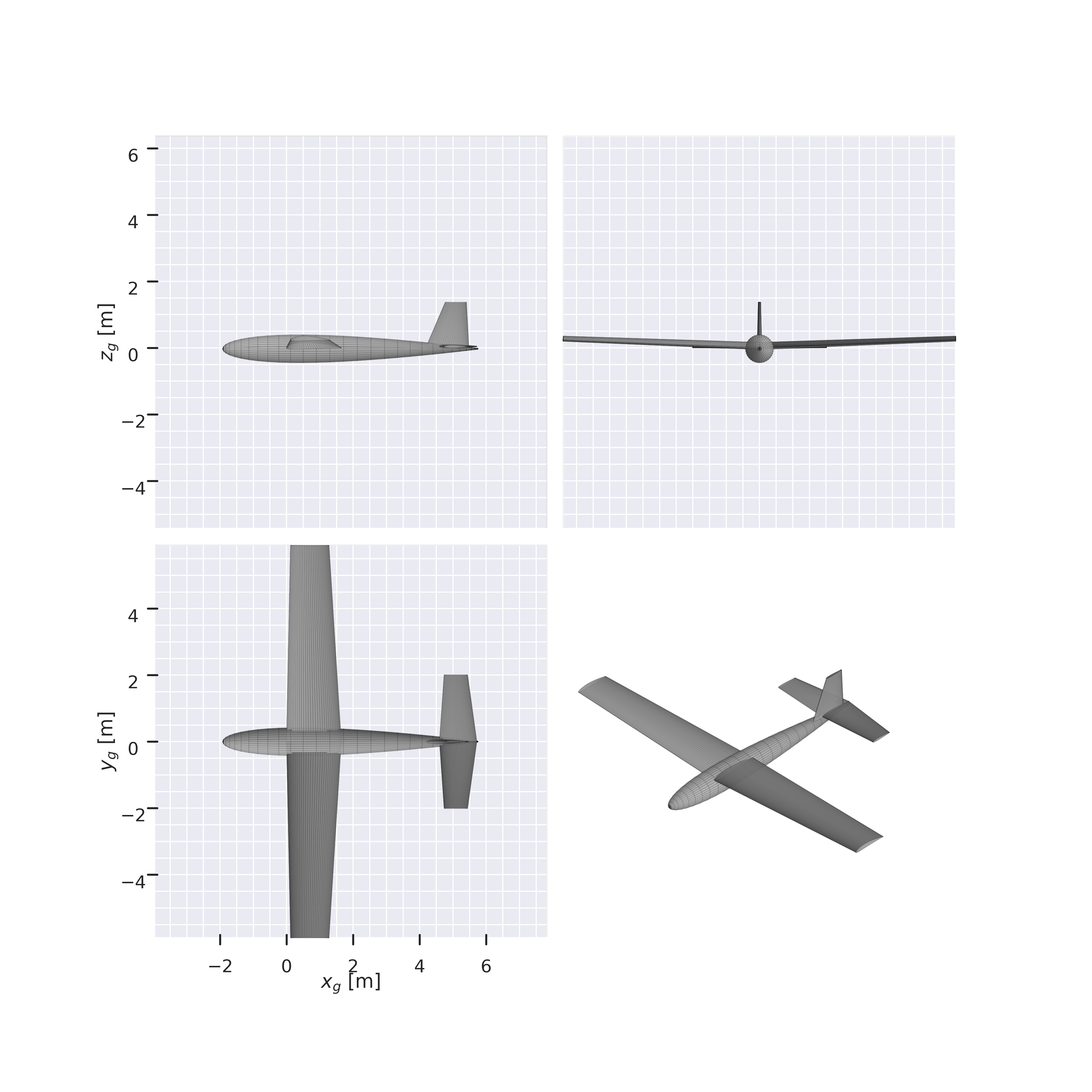
To make the result concrete, Figure 1 wraps the optimized wing in a notional airframe and renders it. The wing’s span and area come straight from the solution; the fuselage and tail are sketched with typical proportions.
Code: build an asb.Airplane around the optimized wing
(a) Three-view of an airplane built around the optimized wing. Span and area are taken directly from the optimization result; fuselage and tail use typical proportions.
And this example scales. The same Opti pattern — declare variables, write physics, add constraints, solve — carries unchanged from five variables to tens of thousands, from a wing sizing study to a full aircraft-plus-trajectory optimization. The rest of this book builds that ladder one rung at a time. (This particular problem gets a much closer look in Wing Design, including the cautionary tale of what happens when you omit the wing weight model.)
0.2 Installation
AeroSandbox requires Python 3.10 or newer, and installs from PyPI:
pip install aerosandbox[full]
The [full] extra installs everything used in this book, including 3D visualization (pyvista), interactive plotting, and CAD-export dependencies. A plain pip install aerosandbox gives a lighter install with all of the optimization, numerics, and physics models but only 2D (matplotlib) plotting. Upgrade any time with pip install --upgrade aerosandbox.
Verify your install:
import aerosandbox as asbprint(asb.__version__)
4.2.9
This book was executed against AeroSandbox 4.2.9 — every code block and every number you see was computed live during rendering, so what you read is what the current library actually does.
0.2.1 Conventions used throughout
Three conventions appear in every chapter, and in essentially all AeroSandbox code in the wild:
The standard imports are import aerosandbox as asb and import aerosandbox.numpy as np. The second one matters: aerosandbox.numpy is a drop-in NumPy replacement that also works on optimization variables, which is what makes models differentiable for free (see Optimization Basics).
Everything is in base SI units (m, kg, s, N, Pa, W, J) unless a variable name says otherwise (e.g., endurance_hours). Since SI is a coherent unit system, quantities combine without conversion factors. For inputs and outputs in other units, use aerosandbox.tools.units as multiplicative conversion factors: airspeed = 100 * u.knot.
The two exceptions: angle of attack alpha and sideslip beta are in degrees, by long-standing aerospace convention. All other angles are radians.
0.3 How this book is organized
The book is a ladder from optimization fundamentals to complete aircraft design studies:
Optimization Foundations (1–3) — the Opti workflow, how to write models the optimizer can’t break (continuity, NaN-safety, scaling), and how to diagnose solves, extract sensitivities, and run design sweeps.
Modeling Aircraft (4–8) — the geometry stack, then physics discipline by discipline: airfoil aerodynamics, whole-aircraft aerodynamics, atmosphere/propulsion/weights, and structures.
Design Optimization (9–10) — putting models in the loop: wing design done wrong and then right, and a complete conceptual aircraft sizing problem.
Trajectory Optimization (11–12) — optimal control by direct collocation, and the flight dynamics class family.
Complete Design Studies (13–15) — three worked designs: an aeroelastic wing, a transport aircraft, and a solar-electric UAV. Multidisciplinary optimization without an MDO framework.
Advanced Topics (16–17) — bringing your own models into the optimizer, and interfacing with external analysis tools.
If you are new to optimization-first design, read Parts I–III in order — the foundations chapters are short and everything downstream leans on them. If you already know a CasADi- or GPkit-style workflow, skim Optimization Basics for syntax and jump to whatever discipline or design study interests you; chapters are written to be readable independently, with cross-references where they lean on earlier material.
API reference:aerosandbox.readthedocs.io hosts complete, auto-generated API documentation. Every public object is also documented in-source: help(asb.Airplane) works, and docstrings include units for all inputs and outputs.
Theory: for the mathematics underpinning the library — automatic differentiation, simultaneous analysis and design, and model transformations — see the author’s PhD thesis, which is effectively the companion theory volume to this practical book.
0.5 Where to go next
Start with Optimization Basics, which unpacks everything the example above glossed over: what opti.variable(), opti.subject_to(), and sol() actually do, and why aerosandbox.numpy lets ordinary-looking code be differentiated exactly. If your interest is modeling airplanes more than optimizing them, Geometry begins the aircraft-modeling thread. And if you’d rather see the destination before the route, the Aerostructural Wing design study shows what a few hundred lines of AeroSandbox can do.