2  Optimization Basics

Everything in AeroSandbox — every airfoil polar, every weight buildup, every trajectory — is designed to sit inside an optimization problem. So before any wings appear, this chapter teaches the machinery that the rest of the book is built on. You will learn the asb.Opti lifecycle (declare variables, add constraints, set an objective, solve, extract values) by working a classic nonconvex benchmark; how to scale from 2 design variables to hundreds using vectorized variables; and why AeroSandbox ships its own drop-in replacement for NumPy. If you internalize this one chapter, every later chapter is “just” writing physics models inside this same five-call pattern.

2.1 The shape of an engineering design problem

Most engineering design problems, reduced to their mathematical skeleton, look surprisingly alike. They are:

• Continuous — the design variables (a wingspan, a cruise altitude) vary smoothly, rather than being discrete choices.
• Nonlinear — the sensitivity of performance to each input changes as you move through the design space.
• Nonconvex — the objective is not always “curving up”, so local information alone can’t certify a global optimum.
• Poorly scaled — variables and their couplings span many orders of magnitude, so the Hessian is ill-conditioned.
• Constrained — the interesting designs live on the boundary of what’s allowed: a structure at its stress limit, a wing at its stall margin.

The classic miniature of the first four properties is the Rosenbrock function — the “Hello, World!” of optimization. Physically, picture a shallow, banana-shaped valley: falling into the valley is easy, but the valley floor is nearly flat along its length and curves as it goes, so following it to the true bottom is hard. In code, it’s one line:

def rosenbrock(x, y):
    return (1 - x) ** 2 + 100 * (y - x**2) ** 2

Here’s what that landscape looks like:

Figure 2.1: Contours of the Rosenbrock function, log-spaced. The minimum hides at the far end of a nearly-flat, curving valley.

With the picture in mind, the problem statement is simply:

\[ \underset{x,\ y}{\text{minimize}} \quad (1-x)^2 + 100\,(y-x^2)^2 \]

The minimum sits at \((1, 1)\), where the function value is exactly zero — a fact we can verify by hand, which makes this a good first test of the machinery.

2.2 The Opti lifecycle

The core of AeroSandbox is the Opti class: an optimization environment where you state a problem in natural mathematical syntax, and a modern gradient-based solver (IPOPT, with derivatives supplied automatically by CasADi) finds the optimum. Under the hood, asb.Opti extends CasADi’s Opti class with engineering-design conveniences — variable scaling, log-transforms, frozen variables — that later chapters will use heavily.

Every Opti problem in this book, from 2 variables to thousands, follows the same five-call lifecycle:

1. opti = asb.Opti() — create an optimization environment.
2. opti.variable(init_guess=...) — declare each design variable, with an initial guess.
3. opti.subject_to(...) — declare constraints (we’ll add one in a moment).
4. opti.minimize(...) — declare the objective.
5. sol = opti.solve(), then sol(...) — solve, and evaluate any expression at the optimum.

Here is the whole lifecycle applied to the Rosenbrock problem:

import aerosandbox as asb  # The standard AeroSandbox import convention

opti = asb.Opti()  # 1. Create an optimization environment

x = opti.variable(init_guess=0)  # 2. Declare variables. Initial guesses are required.
y = opti.variable(init_guess=0)

opti.minimize(rosenbrock(x, y))  # 4. Declare the objective (no constraints yet)

sol = opti.solve()  # 5. Solve.

This is Ipopt version 3.14.11, running with linear solver MUMPS 5.4.1.

Number of nonzeros in equality constraint Jacobian...:        0
Number of nonzeros in inequality constraint Jacobian.:        0
Number of nonzeros in Lagrangian Hessian.............:        3

Total number of variables............................:        2
                     variables with only lower bounds:        0
                variables with lower and upper bounds:        0
                     variables with only upper bounds:        0
Total number of equality constraints.................:        0
Total number of inequality constraints...............:        0
        inequality constraints with only lower bounds:        0
   inequality constraints with lower and upper bounds:        0
        inequality constraints with only upper bounds:        0

iter    objective    inf_pr   inf_du lg(mu)  ||d||  lg(rg) alpha_du alpha_pr  ls
   0  1.0000000e+00 0.00e+00 2.00e+00   0.0 0.00e+00    -  0.00e+00 0.00e+00   0
   1  9.5312500e-01 0.00e+00 1.25e+01 -11.0 1.00e+00    -  1.00e+00 2.50e-01f  3
   2  4.8320569e-01 0.00e+00 1.01e+00 -11.0 9.03e-02    -  1.00e+00 1.00e+00f  1
   3  4.5708829e-01 0.00e+00 9.53e+00 -11.0 4.29e-01    -  1.00e+00 5.00e-01f  2
   4  1.8894205e-01 0.00e+00 4.15e-01 -11.0 9.51e-02    -  1.00e+00 1.00e+00f  1
   5  1.3918726e-01 0.00e+00 6.51e+00 -11.0 3.49e-01    -  1.00e+00 5.00e-01f  2
   6  5.4940990e-02 0.00e+00 4.51e-01 -11.0 9.29e-02    -  1.00e+00 1.00e+00f  1
   7  2.9144630e-02 0.00e+00 2.27e+00 -11.0 2.49e-01    -  1.00e+00 5.00e-01f  2
   8  9.8586451e-03 0.00e+00 1.15e+00 -11.0 1.10e-01    -  1.00e+00 1.00e+00f  1
   9  2.3237475e-03 0.00e+00 1.00e+00 -11.0 1.00e-01    -  1.00e+00 1.00e+00f  1
iter    objective    inf_pr   inf_du lg(mu)  ||d||  lg(rg) alpha_du alpha_pr  ls
  10  2.3797236e-04 0.00e+00 2.19e-01 -11.0 5.09e-02    -  1.00e+00 1.00e+00f  1
  11  4.9267371e-06 0.00e+00 5.95e-02 -11.0 2.53e-02    -  1.00e+00 1.00e+00f  1
  12  2.8189505e-09 0.00e+00 8.31e-04 -11.0 3.20e-03    -  1.00e+00 1.00e+00f  1
  13  1.0095040e-15 0.00e+00 8.68e-07 -11.0 9.78e-05    -  1.00e+00 1.00e+00f  1
  14  1.3288608e-28 0.00e+00 2.02e-13 -11.0 4.65e-08    -  1.00e+00 1.00e+00f  1

Number of Iterations....: 14

                                   (scaled)                 (unscaled)
Objective...............:   1.3288608467480825e-28    1.3288608467480825e-28
Dual infeasibility......:   2.0183854587685121e-13    2.0183854587685121e-13
Constraint violation....:   0.0000000000000000e+00    0.0000000000000000e+00
Variable bound violation:   0.0000000000000000e+00    0.0000000000000000e+00
Complementarity.........:   0.0000000000000000e+00    0.0000000000000000e+00
Overall NLP error.......:   2.0183854587685121e-13    2.0183854587685121e-13


Number of objective function evaluations             = 36
Number of objective gradient evaluations             = 15
Number of equality constraint evaluations            = 0
Number of inequality constraint evaluations          = 0
Number of equality constraint Jacobian evaluations   = 0
Number of inequality constraint Jacobian evaluations = 0
Number of Lagrangian Hessian evaluations             = 14
Total seconds in IPOPT                               = 0.026

EXIT: Optimal Solution Found.
      solver  :   t_proc      (avg)   t_wall      (avg)    n_eval
       nlp_f  |   1.42ms ( 39.56us) 239.45us (  6.65us)        36
  nlp_grad_f  | 569.00us ( 35.56us) 110.70us (  6.92us)        16
  nlp_hess_l  | 693.00us ( 49.50us) 160.27us ( 11.45us)        14
       total  | 199.18ms (199.18ms)  26.87ms ( 26.87ms)         1

The solver prints a progress log as it works. For now, only the last lines matter: EXIT: Optimal Solution Found means the solver converged to a point satisfying the optimality conditions, and the timing table shows the entire solve took milliseconds (re-timing this solve on this machine gives about 25 ms, in 14 iterations). We’ll learn to read the rest of this log — and what to do when it doesn’t say “Optimal Solution Found” — in Chapter 5.

Note two things about the code. First, rosenbrock() is an ordinary Python function, written before opti existed — you can organize your models with functions and classes as usual, and pass optimization variables through them. Second, extracting answers uses sol(...), which evaluates any expression at the optimum, not just bare variables:

print(f"x = {sol(x)}")
print(f"y = {sol(y)}")
print(f"objective = {sol(rosenbrock(x, y))}")

x = 0.9999999999999899
y = 0.9999999999999792
objective = 1.3288608467480825e-28

The solver lands on \((1, 1)\) to machine precision, matching the hand calculation.

NoteInitial guesses

init_guess tells the optimizer where to start looking. For this small problem almost any start works, but for large nonconvex problems the quality of your initial guess strongly affects both solve time and which local optimum you find. Get in the habit of providing physically-sensible guesses.

2.3 Adding a constraint

Real design problems are constrained, so let’s constrain this one: find the lowest point of the Rosenbrock valley that lies within the unit circle, i.e. subject to \(x^2 + y^2 \le 1\). The unconstrained minimum at \((1, 1)\) has a radius of \(\sqrt{2}\), so it’s no longer feasible — we expect the new optimum to sit on the circle, somewhere down-valley of \((1, 1)\).

Constraints are declared with opti.subject_to(), using natural comparison syntax. We’ll also start the solver at \((-1.5, 1.5)\) — deliberately outside the feasible circle — to make a point: initial guesses do not need to be feasible. IPOPT drives infeasibility to zero as it converges.

One new trick here: opti.solve() accepts a callback function that runs at every solver iteration. Inside it, opti.debug.value(...) reads the current (not-yet-converged) value of any expression — ideal for recording the optimizer’s path so we can watch it think:

opti = asb.Opti()

x = opti.variable(init_guess=-1.5)
y = opti.variable(init_guess=1.5)  # Note: (-1.5, 1.5) is infeasible. That's fine.

opti.minimize(rosenbrock(x, y))

opti.subject_to(x**2 + y**2 <= 1)  # Constrain the design to the unit disk

iterates = []  # Record the optimizer's path, for plotting

sol = opti.solve(
    callback=lambda iteration: iterates.append(
        (opti.debug.value(x), opti.debug.value(y))
    ),
    verbose=False,  # Suppresses the IPOPT log we saw earlier
)

x_star, y_star = sol(x), sol(y)
r_star = sol((x**2 + y**2) ** 0.5)
print(f"Optimum: x = {x_star:.6f}, y = {y_star:.6f}, radius = {r_star:.6f}")

Optimum: x = 0.786415, y = 0.617698, radius = 1.000000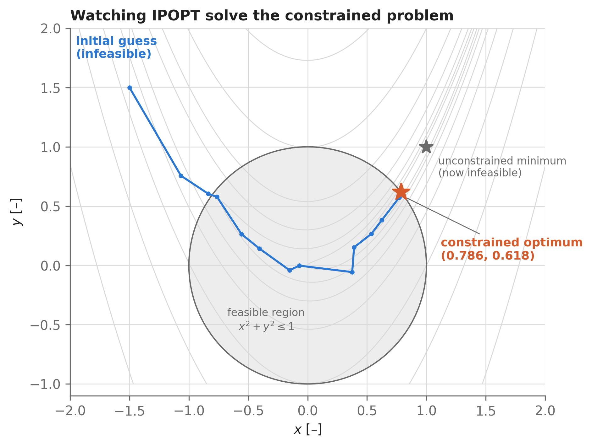

Figure 2.2: The optimizer’s path on the constrained Rosenbrock problem. Starting from an infeasible guess, IPOPT steps into the feasible disk, finds the valley floor, and follows it until the constraint stops it.

The optimum lands at (0.786, 0.618), and its radius is 1.000000 — the constraint is active (tight) at the solution, exactly as the geometry suggested. The whole 18-iteration solve, path recording included, still takes milliseconds. (If you wanted to certify this optimum by hand, you’d verify the KKT conditions; for now, we’ll trust the optimizer’s convergence test, which checks exactly that.)

A few practical notes on constraints:

• Strict vs. non-strict inequalities are the same thing here. Numerically, there’s no difference between < and <= (or > and >=) — use whichever reads better.
• Equality constraints use ==. For example, opti.subject_to(lift == weight) is the standard way to close a steady-flight force balance — you’ll see this constantly from Chapter 10 onward.
• You can pass a list. opti.subject_to([x >= 0, x <= 5]) declares both constraints at once; this often makes model code read like a specification.
• Declaration order is free. Variables, constraints, and the objective can be declared in any order, as long as everything is in place before opti.solve().
• opti.maximize(f) exists too — it’s simply sugar for opti.minimize(-f).

2.4 Vectorized variables

Declaring variables one at a time stops scaling long before real problems do — a trajectory optimization might need the aircraft’s altitude at 100 points in time. Rule #1 of scientific Python applies to optimization too: vectorize everything. opti.variable() creates a whole vector of decision variables when you hand it a vector initial guess.

The standard benchmark here is the \(N\)-dimensional sphere problem — words first: find the point closest to the origin, where “closeness” is the sum of squared coordinates. As math:

\[ \underset{\vec{x}}{\text{minimize}} \quad \sum_{i=1}^{N} x_i^2 \]

Let’s solve it in 100-dimensional space:

import aerosandbox.numpy as np  # More on this import in the next section!

N = 100

opti = asb.Opti()

x = opti.variable(init_guess=np.ones(N))  # A vector variable: length inferred
                                          # from the initial guess.
opti.minimize(np.sum(x**2))

sol = opti.solve(verbose=False)

print(f"Number of variables:  {N}")
print(f"Solver iterations:    {sol.stats()['iter_count']}")
print(f"Max |x_i| at optimum: {np.max(np.abs(sol(x))):.2e}")

Number of variables:  100
Solver iterations:    1
Max |x_i| at optimum: 0.00e+00

All 100 components go to zero — in a single solver iteration. That’s no accident: the sphere problem is an unconstrained quadratic, and IPOPT is a second-order (Newton-type) method, so one full Newton step lands exactly on the optimum. This is a recurring theme: modern solvers exploit curvature information, and (as we’ll see next) AeroSandbox supplies exact second derivatives automatically.

Vector variables really shine because constraints broadcast element-wise, just like NumPy arithmetic. One subject_to() call below creates 100 constraints — a per-element lower bound \(x_i \ge b_i\):

b = np.linspace(-1, 1, N)  # A different lower bound for each element

opti = asb.Opti()
x = opti.variable(init_guess=np.ones(N))
opti.subject_to(x >= b)  # 100 constraints in one line
opti.minimize(np.sum(x**2))

sol = opti.solve(verbose=False)
x_opt = sol(x)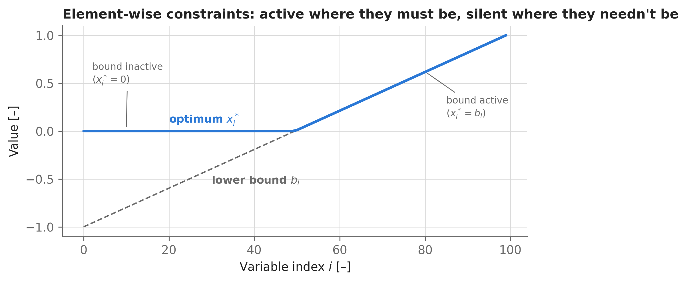

Figure 2.3: Solution of the bounded sphere problem. Where the lower bound is negative, the optimizer parks each element at its unconstrained optimum of zero; where the bound is positive, the constraint is active and the element sits exactly on it.

The result reads like a textbook illustration of constrained optimality: each element independently settles at \(\max(b_i,\, 0)\). Where the bound doesn’t bind, the optimizer ignores it; where it does, the solution sits exactly on it.

More syntax you’ll use constantly:

• Scalar guess, explicit length: opti.variable(init_guess=1, n_vars=N) is shorthand for a length-N vector with every element initialized to 1. Use the array form (init_guess=np.linspace(...)) when elements should start at different values — for trajectory problems, a straight-line guess between endpoints is a great default.
• Indexing works: x[3], x[10:20], and friends behave as you’d expect, so you can constrain, say, boundary conditions: opti.subject_to(x[0] == 0).
• Dimensionality: scalars and 1D vectors cover nearly all engineering design problems; 2D matrix variables are supported, but higher-dimensional arrays of decision variables are not (plain aerosandbox.numpy math on numeric arrays has no such limit).

2.5 Why aerosandbox.numpy exists

You may have noticed the import import aerosandbox.numpy as np above and wondered why we don’t just use NumPy. The short answer: so that the solver can differentiate your code.

Here’s the chain of reasoning. IPOPT is a gradient-based optimizer: at every iteration it needs derivatives of the objective and every constraint with respect to every variable — including exact second derivatives, which is how the sphere problem solved in one Newton step. Computing those by finite differences would be slow and noisy; deriving them by hand, for an entire aircraft model, would be unthinkable. Instead, CasADi uses automatic differentiation (AD): when you write rosenbrock(x, y) with opti variables, no arithmetic actually happens — instead, a symbolic trace (a directed graph of every +, *, cos, exp, …) is recorded, and exact derivatives of the whole graph come almost for free. This is why an opti variable prints as a symbolic MX object rather than a number.

The catch: every operation between variable and objective must be traceable. Plain NumPy functions don’t know what a CasADi MX object is, so they would break the trace (or crash). Rewriting your math in CasADi’s own syntax would work, but then your model code couldn’t be run on ordinary numbers. AeroSandbox resolves this with a dual-backend NumPy: aerosandbox.numpy re-exports all of NumPy, and re-implements the functions that need it so that each one dispatches on its input type —

• NumPy arrays in → NumPy arrays out, with identical behavior and speed to stock NumPy;
• Optimization variables in → traced symbolic expressions out, keeping the AD graph intact.

So the practice is simply: in any code that might ever touch an optimization variable, write import aerosandbox.numpy as np instead of import numpy as np — and then write your engineering models once, use them everywhere. Let’s see the dispatch in action with np.where, the vectorized if/else:

import aerosandbox.numpy as np

# Numeric inputs: behaves exactly like numpy.where...
values = np.linspace(0, 4, 5)
print(np.where(values > 2, values, 0.0))
print(type(np.where(values > 2, values, 0.0)))

[0. 0. 0. 3. 4.]
<class 'numpy.ndarray'>

# ...symbolic inputs: builds a traceable expression instead.
opti = asb.Opti()
v = opti.variable(init_guess=1)

expression = np.where(v > 2, v, 0.0)
print(type(expression))

<class 'casadi.casadi.MX'>

Same function, same call signature — a NumPy ndarray in the first case, a symbolic CasADi MX node in the second. Every AeroSandbox physics model is built out of functions like this, which is why the same drag model can be evaluated on a plain float for a quick check and optimized through with exact gradients.

aerosandbox.numpy also adds functions stock NumPy doesn’t have, purpose-built for optimization. A favorite is np.softmax — a smooth, differentiable stand-in for max(). It’s worth a picture: the hard maximum has a kink where the two arguments cross, and gradient-based optimizers handle kinks badly. softmax rounds the kink off, with a softness parameter (in the same units as the inputs) setting how much discrepancy between the inputs is “physically significant”:

t = np.linspace(-2, 2, 300)
hard = np.maximum(t, 0)
soft = np.softmax(t, 0, softness=0.4)  # Works on arrays...
print(f"softmax(3, 4) = {np.softmax(3, 4, softness=0.4):.4f}")  # ...and scalars.

softmax(3, 4) = 4.0316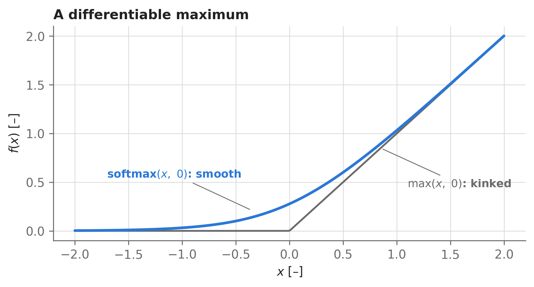

Figure 2.4: The hard maximum has a kink at the crossover; softmax rounds it off so gradient-based optimizers always see smooth curvature.

And because np.softmax is smooth and traceable, you can optimize straight through it — here, finding the point where two crossing lines have the lowest “soft-maximum”, a miniature of the min-max problems that appear constantly in design (e.g., minimizing the worst-case drag across flight conditions):

opti = asb.Opti()
v = opti.variable(init_guess=3)

worst_case = np.softmax(v, 2 - v, softness=0.5)  # Smooth max of two functions
opti.minimize(worst_case)

sol = opti.solve(verbose=False)
print(f"v = {sol(v):.4f}, worst-case value = {sol(worst_case):.4f}")

v = 1.0000, worst-case value = 1.3466

The optimizer settles at v = 1.00, right at the crossover — precisely where a hard max() would have a non-differentiable kink and stall a naive formulation. (The full playbook of such reformulation tricks — and the sharp edges of np.where, which is traceable but still kinked — is the subject of Chapter 3.)

The catalog of traceable operations is extensive: trigonometry, logarithms, interpolation, norms, linear solves, and more. Not every obscure NumPy function has been overloaded, though — if something you need is missing, check aerosandbox/numpy/test_numpy/test_all_operations_run.py for what’s supported, and open an issue for what isn’t.

2.6 Where to go next

You now have the complete Opti vocabulary: variable / subject_to / minimize / solve / sol(), vectorized, with aerosandbox.numpy keeping everything differentiable. Three good directions from here:

• Chapter 3 teaches the modeling patterns that keep real problems solvable — continuity and differentiability tricks, NaN-proofing, and problem scaling. Read it before writing your first serious model; it’s the difference between solves that converge and solves that mysteriously don’t.
• Chapter 5 goes deeper on the solve itself: reading IPOPT’s output, solver options, parameter sweeps, and extracting sensitivities (dual variables) from a converged solution.
• Impatient for airplanes? Chapter 10 applies exactly the machinery from this chapter to a real wing design problem — including a cautionary tale about what optimizers do to under-constrained models.