import aerosandbox as asb
import aerosandbox.numpy as np

# Physical constants, in base SI units (AeroSandbox convention -- no exceptions):
density = 1.225      # air density [kg/m^3]
viscosity = 1.81e-5  # air dynamic viscosity [kg/(m*s)]
weight = 100         # payload weight [N], about 10 kg

opti = asb.Opti()

aspect_ratio = opti.variable(init_guess=10, log_transform=True)
wing_area = opti.variable(init_guess=1, log_transform=True) # [m^2]10 Wing Design: A Cautionary Tale
This chapter is your first real design problem: size a wing to lift a payload with as little drag as possible. We solve it twice. The first formulation is bug-free code that converges in milliseconds — to a wing with an aspect ratio of about 300 that would snap like dry spaghetti in the first gust. The second adds three pieces of honest physics (wing weight, fuselage drag, and a takeoff constraint) and lands on a thoroughly sensible airplane. The distance between those two answers is the most important lesson in design optimization: the optimizer answers exactly the question you pose, which is not necessarily the question you meant to pose. By the end of the chapter, you will know how to recognize a model that cannot push back against the optimizer — and how to fix one that can’t.
We assume you’re comfortable with the asb.Opti workflow (variable → subject_to → minimize → solve) from Section 2.1.
10.1 The problem
Suppose we need to carry a payload of about 10 kg — a weight of 100 N — in steady, level flight at sea level. We get to choose the wing’s size, its shape, and the speed at which we fly. To keep this first pass simple, we assume the wing is rectangular and (here comes the loaded gun) massless.
A rectangular planform is fully described by two numbers. Span \(b\) and chord \(c\) would work, but we’ll instead use aspect ratio \(AR = b^2/S\) and wing area \(S\) — the pair is equivalent, and it has two minor advantages: aspect ratio is nondimensional (which helps with scaling), and our aerodynamic quantities of interest (lift, induced drag) connect more directly to \(AR\) and \(S\) than to \(b\) and \(c\).
Both variables are declared with log_transform=True: internally, the optimizer works with \(\ln(S)\) rather than \(S\) itself. This guarantees positivity for free (no constraint needed), often improves scaling, and can make design problems more convex — many aircraft-design relations are power laws, which turn linear under a log transform. It’s not a free lunch (the transform is itself a nonlinearity), and we discuss when to reach for it in Chapter 3. Here it mostly serves as an introduction to the concept.
We also don’t know the best airspeed to fly at, so we leave that to the optimizer too:
airspeed = opti.variable(init_guess=30, lower_bound=0) # [m/s]Airspeed is another always-positive quantity, so we could have log-transformed it as well; instead, we use the lower_bound argument to show a second way of keeping a variable nonnegative. (It’s exactly equivalent to writing opti.subject_to(airspeed > 0) yourself.)
10.2 A naive drag model
Wing drag has two main contributions. Profile drag comes from the viscous boundary layer scrubbing along the surface; the simplest possible model is the skin friction of a laminar flat plate (the Blasius solution), which depends only on the chord Reynolds number. Induced drag is the price of generating lift with a finite span: the wing leaves behind a vortex wake, and for the ideal (elliptical) spanwise lift distribution, the induced drag coefficient depends only on \(C_L\) and aspect ratio. In symbols:
\[ C_D \;=\; \underbrace{\frac{1.328}{\sqrt{\mathrm{Re}_c}}}_{\text{profile (laminar flat plate)}} \;+\; \underbrace{\frac{C_L^2}{\pi \, AR}}_{\text{induced (elliptical loading)}}, \qquad D = q \, S \, C_D \]
where \(q = \tfrac{1}{2}\rho V^2\) is dynamic pressure. Steady level flight requires lift to equal weight, and we’ll keep the wing out of stall by bounding \(|C_L| \le 1.2\). That’s the whole model:
span = (aspect_ratio * wing_area) ** 0.5  # from AR = b^2 / S
chord = span / aspect_ratio

dynamic_pressure = 0.5 * density * airspeed**2
lift = weight  # steady level flight
CL = lift / dynamic_pressure / wing_area

Re = density * airspeed * chord / viscosity
CD_profile = 1.328 * Re**-0.5           # Blasius laminar flat plate
CD_induced = CL**2 / (np.pi * aspect_ratio)  # elliptical lift distribution
CD = CD_profile + CD_induced
drag = dynamic_pressure * wing_area * CD

opti.subject_to([
    CL < 1.2,   # stall
    CL > -1.2,  # stall
])
opti.minimize(drag)

sol = opti.solve(verbose=False)

print(f"Minimum drag: {sol(drag):.3f} N")
print(f"Aspect ratio: {sol(aspect_ratio):.1f}")
print(f"Wing area:    {sol(wing_area):.3f} m^2")
print(f"Airspeed:     {sol(airspeed):.1f} m/s")
print(f"Lift-to-drag: {sol(lift / drag):.1f}")
Minimum drag: 0.646 N
Aspect ratio: 295.8
Wing area: 0.099 m^2
Airspeed: 37.0 m/s
Lift-to-drag: 154.9IPOPT converges in a handful of iterations, and the news is spectacular: only 0.65 N of drag to lift 100 N of payload — a lift-to-drag ratio of 155. For reference, the best open-class competition sailplanes ever built, with 25+ meters of exquisitely-crafted wing, achieve an \(L/D\) of about 70. Either we’ve just doubled the state of the art with ten lines of Python, or something is deeply wrong.
Look at the wing the optimizer chose:
Show plotting code
import _common
import matplotlib.pyplot as plt

b_opt, c_opt, S_opt = sol(span), sol(chord), sol(wing_area)
AR_naive_opt = sol(aspect_ratio)
b_ref = (8 * S_opt) ** 0.5  # a conventional AR = 8 wing of the same area
c_ref = S_opt / b_ref

fig, ax = plt.subplots(figsize=(9, 2.4))
ax.add_patch(
    plt.Rectangle((-b_opt / 2, 0), b_opt, c_opt, facecolor=_common.SERIES[3])
)
ax.add_patch(
    plt.Rectangle((-b_ref / 2, -0.5), b_ref, c_ref, facecolor=_common.TEXT_SECONDARY)
)
ax.text(
    0, 0.10,
    f'the "optimal" wing:  span {b_opt:.1f} m,  chord {c_opt * 1e3:.0f} mm,'
    f'  AR {sol(aspect_ratio):.0f}',
    color=_common.SERIES[3], ha="center", fontweight="bold", fontsize=10,
)
ax.text(
    0, -0.5 + c_ref + 0.08,
    f"an AR = 8 wing of equal area, for scale",
    color=_common.TEXT_SECONDARY, ha="center", fontweight="bold", fontsize=10,
)
ax.set_aspect("equal")
ax.set_xlim(-3.1, 3.1)
ax.set_ylim(-0.62, 0.35)
ax.set_yticks([])
ax.spines["left"].set_visible(False)
ax.grid(False)
ax.set_xlabel("Spanwise position [m]")
plt.show()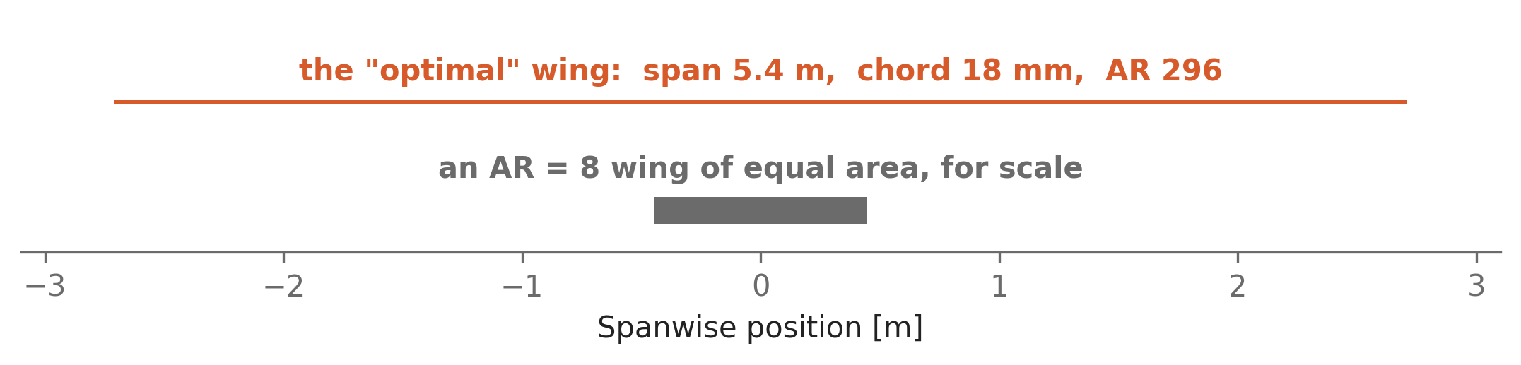
This “airplane” carries 10 kg on a wing with the proportions of a strand of fettuccine. The solution report is full of red flags once you know where to look:
- A design variable ran to an absurd extreme. An aspect ratio of 296 means a 5.4 m span with a chord of 18 mm. Nothing in the model made this expensive.
- A performance metric beats the physical state of the art by 2×. When your ten-line model outperforms every sailplane ever built, the burden of proof is on the model.
- A variable is pinned against a bound you added “for realism.” The optimized \(C_L\) is 1.2000 — hard against the stall bound of 1.2. As we’ll see below, that’s a symptom, not a coincidence.
- The solution isn’t even unique. Watch what happens if we re-solve the same problem from different initial guesses for airspeed:
areas = []
for airspeed_guess in [20, 30, 60]:
    opti.set_initial(airspeed, airspeed_guess)
    sol_i = opti.solve(verbose=False)
    areas.append(sol_i(wing_area))
    print(
        f"initial guess {airspeed_guess} m/s -> "
        f"drag = {sol_i(drag):.6f} N  |  "
        f"wing area = {sol_i(wing_area):.3f} m^2  |  "
        f"airspeed = {sol_i(airspeed):.1f} m/s"
    )
initial guess 20 m/s -> drag = 0.645678 N | wing area = 0.166 m^2 | airspeed = 28.6 m/s
initial guess 30 m/s -> drag = 0.645678 N | wing area = 0.099 m^2 | airspeed = 37.0 m/s
initial guess 60 m/s -> drag = 0.645678 N | wing area = 0.036 m^2 | airspeed = 61.1 m/sIdentical drag to six decimal places, from wing areas that differ by a factor of 4.6. The lift constraint fixes the product \(q \, S\) at a given \(C_L\), and it happens that in this model the Reynolds number then depends only on \(AR\) and \(C_L\) — so drag is completely indifferent to how we split \(q \, S\) between flying fast with a small wing or slow with a big one. The optimizer is wandering a perfectly flat valley in the design space and stopping wherever it pleases. A model with a flat direction in it is a model with missing physics: reality always has an opinion about airspeed.
10.3 The autopsy
Here is the uncomfortable part: the optimizer did nothing wrong. Every number above is the mathematically correct answer to the question we asked. We just asked a question whose honest answer is a fettuccine glider. Specifically:
The wing weighs nothing. In reality, the reason nobody builds an aspect ratio of 300 is structural: bending loads grow brutally with span, so more slender means heavier, and heavier means more lift needed, and more lift means more drag. We deleted that entire feedback loop when we said “assume the wing is massless.” The only thing in our model that resisted slenderness at all was a whisper of Reynolds-number physics — as \(AR\) rises at fixed area, the chord shrinks, \(\mathrm{Re}\) falls (it’s roughly 46,000 at the optimum — model-airplane scale), and the Blasius \(C_f\) creeps upward. That second-order effect is the only reason the answer was 296 rather than infinity.
Profile drag is blind to lift. Our flat-plate skin friction doesn’t depend on \(C_L\) at all, and at \(AR \approx 300\) the induced drag is nearly gone. So lift is essentially free — and if lift is free, you take all of it you’re allowed. That’s why \(C_L\) slammed into the 1.2 stall bound: the bound is doing work that the physics should have been doing (real airfoils get draggy near stall — see Chapter 6).
There is no airplane attached to this wing. No fuselage drag, no tail, no propulsion penalty. That absence is exactly the flat valley from red flag #4: nothing in the model cares how fast we fly.
There is no off-design requirement. Real wings must also take off, land, and tolerate gusts — all of which push toward more area and less slenderness.
Note something subtle about the first point: it is not enough to model the effect; you must model the dependence that creates the trade. Adding a wing mass proportional to wing area would change the numbers but not the nonsense — the optimizer would still crank the aspect ratio sky-high, because area-proportional mass doesn’t penalize slenderness. The mass model must know about span and aspect ratio, because that dependence is the physics that kills fettuccine wings.
When an optimizer hands you a suspicious design, the most productive question is: “Why wouldn’t this actually work in real life?” Whatever your answer — “the wing would snap,” “it can’t take off,” “that L/D is fantasy” — points directly at the constraint you forgot or the assumption you didn’t realize you were making. If a weird answer appears, 99 times out of 100 it’s a problem with the question, not with the optimizer.
10.4 Asking the right question
Now let’s fix the model. This formulation follows a classic benchmark problem from Hoburg and Abbeel’s Geometric Programming for Aircraft Design Optimization (Section 3), with constants matched to the GPKit “simple wing” example. The airplane is now a small kit-plane-class machine with a fixed fuselage, and the model gains exactly the physics whose absence we diagnosed above:
- A wing weight model. Two terms: a surface term proportional to area (skin, ribs), and a structural term from root bending. Words first: the bending moment at the wing root grows with span; the structure’s depth available to react it is the airfoil thickness \(\tau \, c\); working through a beam-sizing argument (Hoburg & Abbeel give the derivation) yields a structural weight scaling like
\[ W_\mathrm{wing} = \underbrace{45.24 \,[\mathrm{Pa}] \cdot S}_{\text{surface: skin, ribs}} \;+\; \underbrace{8.71 \times 10^{-5}\,[\mathrm{m^{-1}}] \cdot \frac{N \; AR^{1.5} \sqrt{W_0 \, W \, S}}{\tau}}_{\text{structure: root bending}} \]
where \(N\) is the ultimate load factor, \(W_0\) the fixed (non-wing) weight, and \(W\) the total weight. The \(AR^{1.5}\) is the pushback we were missing. Notice that total weight \(W\) appears inside its own buildup — weight closure is an implicit equation. In AeroSandbox we don’t need an iterative “sizing loop” for this: we simply declare \(W\) a variable and hand the closure to the optimizer as a constraint. This trick carries entire aircraft sizing problems, as we’ll see in Chapter 11.
Fuselage drag, as a fixed drag area \((C_D A)_\mathrm{fuse} = 0.031\ \mathrm{m^2}\). Now flying faster costs something, and the flat valley in airspeed disappears.
A takeoff constraint: at 22 m/s with flaps down (\(C_{L,\max} = 1.5\)), the wing must lift the whole airplane. Now shrinking the wing costs something.
Less flattering aerodynamics: turbulent flat-plate skin friction (\(C_f = 0.074/\mathrm{Re}^{0.2}\), Schlichting) with a form factor and a wetted-area ratio, and an Oswald efficiency of 0.95 on the induced drag. No more laminar fantasies at flight Reynolds numbers.
### Constants
form_factor = 1.2                   # pressure-drag form factor [-]
oswalds_efficiency = 0.95           # Oswald efficiency factor [-]
viscosity = 1.78e-5                 # air dynamic viscosity [kg/(m*s)]
density = 1.23                      # air density [kg/m^3]
airfoil_thickness_fraction = 0.12   # airfoil thickness / chord [-]
ultimate_load_factor = 3.8          # ultimate structural load factor [-]
airspeed_takeoff = 22.0             # takeoff speed [m/s]
CL_max = 1.5                        # maximum CL, flaps down [-]
wetted_area_ratio = 2.05            # wetted area / reference area [-]
W_W_coeff1 = 8.71e-5                # wing weight coefficient 1 [1/m]
W_W_coeff2 = 45.24                  # wing weight coefficient 2 [Pa]
drag_area_fuselage = 0.031          # fuselage drag area [m^2]
weight_fuselage = 4940.0            # weight excluding wing [N]
We’ll wrap the design problem in a function this time. This is the cheapest trade-study infrastructure you will ever build: a function whose inputs are the parameters you might want to sweep, and whose output is the solved design. (The optional aspect_ratio argument freezes that variable to a given value — we’ll use it shortly. The optional init_guesses lets us warm-start from a neighboring solution, a trick covered properly in Chapter 5.)
def design_wing(aspect_ratio=None, init_guesses=None):
    """Minimum-cruise-drag wing design.

    If `aspect_ratio` is None, it is a design variable; otherwise it is
    held fixed at the given value.
    """
    guess = dict(wing_area=10, airspeed=100, weight=10000, CL=1)
    guess.update(init_guesses or {})

    opti = asb.Opti()

    ### Variables (all positive-by-physics, so all log-transformed)
    AR = (
        opti.variable(init_guess=10, log_transform=True)
        if aspect_ratio is None
        else aspect_ratio
    )
    wing_area = opti.variable(init_guess=guess["wing_area"], log_transform=True)
    airspeed = opti.variable(init_guess=guess["airspeed"], log_transform=True)
    weight = opti.variable(init_guess=guess["weight"], log_transform=True)
    CL = opti.variable(init_guess=guess["CL"], log_transform=True)

    ### Aerodynamics
    CD_fuselage = drag_area_fuselage / wing_area
    Re = (density / viscosity) * airspeed * (wing_area / AR) ** 0.5
    Cf = 0.074 / Re**0.2  # turbulent flat plate (Schlichting)
    CD_profile = form_factor * Cf * wetted_area_ratio
    CD_induced = CL**2 / (np.pi * AR * oswalds_efficiency)
    CD = CD_fuselage + CD_profile + CD_induced
    dynamic_pressure = 0.5 * density * airspeed**2
    drag = dynamic_pressure * wing_area * CD

    lift_cruise = dynamic_pressure * wing_area * CL
    lift_takeoff = 0.5 * density * wing_area * CL_max * airspeed_takeoff**2

    ### Wing weight buildup
    weight_wing = W_W_coeff2 * wing_area + (
        W_W_coeff1 * ultimate_load_factor * AR**1.5
        * (weight_fuselage * weight * wing_area) ** 0.5
    ) / airfoil_thickness_fraction

    opti.subject_to([
        weight <= lift_cruise,                    # can cruise
        weight <= lift_takeoff,                   # can take off
        weight == weight_fuselage + weight_wing,  # weight closure
    ])
    opti.minimize(drag)

    sol = opti.solve(verbose=False)
    return sol, {
        "aspect_ratio": AR, "wing_area": wing_area, "airspeed": airspeed,
        "weight": weight, "CL": CL, "drag": drag, "weight_wing": weight_wing,
        "D_fuselage": dynamic_pressure * wing_area * CD_fuselage,
        "D_profile": dynamic_pressure * wing_area * CD_profile,
        "D_induced": dynamic_pressure * wing_area * CD_induced,
    }


sol, wing = design_wing()| Quantity | Optimum | Units |
|---|---|---|
| Drag (objective) | 303.1 | N |
| Aspect ratio | 8.46 | – |
| Wing area | 16.4 | m² |
| Span | 11.8 | m |
| Chord | 1.39 | m |
| Cruise airspeed | 38.2 | m/s |
| Cruise lift coefficient | 0.499 | – |
| Gross weight | 7341 | N |
| … of which wing | 2401 | N |
| Lift-to-drag ratio | 24.2 | – |
Every symptom from the autopsy is cured. The aspect ratio is 8.5 — a normal airplane, not a noodle. The lift coefficient is 0.50, sitting at an interior optimum rather than pinned against a bound: induced drag now genuinely punishes high \(C_L\). The \(L/D\) of 24.2 is still a touch optimistic (there’s no tail, no interference drag, and the flat-plate profile model flatters real wings), but it’s the right order of magnitude for a clean design. And the wing is 33% of gross weight — the structure now has a real seat at the table.
Airspeed is no longer a matter of indifference, either. Freeze the optimized airplane (its weight, area, and aspect ratio) and sweep cruise speed, and you get the classic drag bucket:
Show plotting code
import _common
import matplotlib.pyplot as plt

W_opt = sol(wing["weight"])
S_opt = sol(wing["wing_area"])
AR_opt = sol(wing["aspect_ratio"])
V_opt, D_opt = sol(wing["airspeed"]), sol(wing["drag"])

V_stall = (2 * W_opt / (density * S_opt * CL_max)) ** 0.5
V = np.linspace(V_stall, 70, 300)
q = 0.5 * density * V**2
CL_cruise = W_opt / (q * S_opt)  # lift = weight fixes CL at each speed
Re = (density / viscosity) * V * (S_opt / AR_opt) ** 0.5

D_fuselage = q * drag_area_fuselage
D_profile = q * S_opt * form_factor * (0.074 / Re**0.2) * wetted_area_ratio
D_induced = q * S_opt * CL_cruise**2 / (np.pi * AR_opt * oswalds_efficiency)
D_total = D_fuselage + D_profile + D_induced

fig, ax = plt.subplots(figsize=(8, 4.2))
for D, name, color in [
    (D_induced, "induced", _common.TEXT_SECONDARY),
    (D_profile, "wing profile", _common.TEXT_SECONDARY),
    (D_fuselage, "fuselage", _common.TEXT_SECONDARY),
]:
    ax.plot(V, D, color=color, linewidth=1.2)
    _common.label_line(ax, V[-1], D[-1], f" {name}", color)
ax.plot(V, D_total, color=_common.SERIES[0])
_common.label_line(ax, V[-1], D_total[-1], " total", _common.SERIES[0])
ax.plot(V_opt, D_opt, "o", color=_common.SERIES[0], markersize=7, zorder=5)
ax.annotate(
    f"optimum: {D_opt:.0f} N at {V_opt:.1f} m/s",
    xy=(V_opt, D_opt), xytext=(V_opt + 2, D_opt - 60),
    color=_common.SERIES[0], fontweight="bold", fontsize=9,
)
_common.annotate_event(ax, V_stall, f"stall at CL_max ({V_stall:.0f} m/s)")
ax.set_xlim(20, 76)
ax.set_xlabel("Cruise airspeed [m/s]")
ax.set_ylabel("Drag [N]")
plt.show()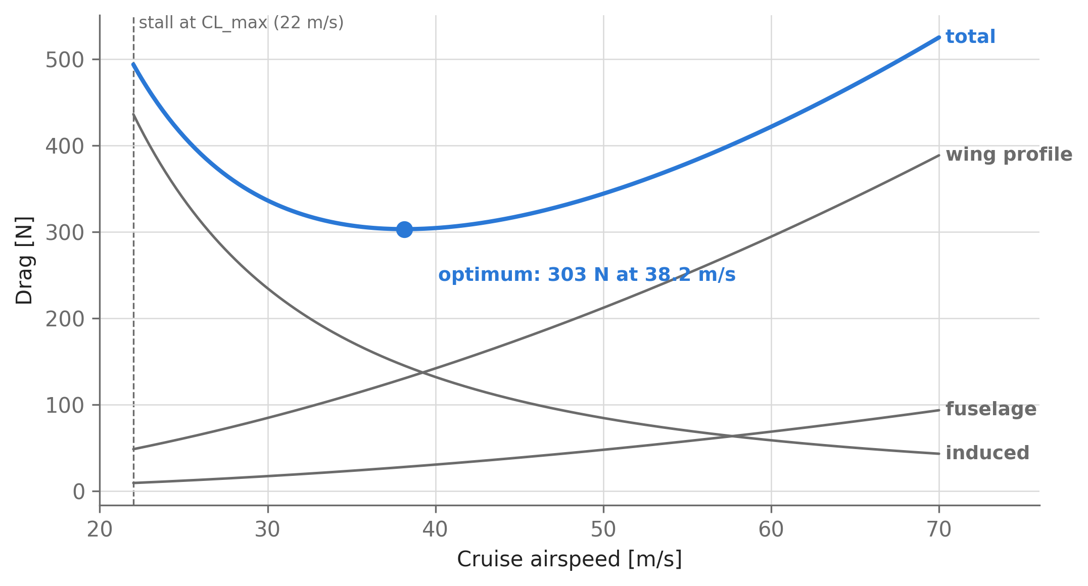
At the optimum, the drag breakdown is 145 N induced, 130 N wing profile, and 28 N fuselage — induced drag roughly balancing everything else, as classical performance theory predicts for a minimum-drag cruise condition. None of this structure existed in the naive model: there, this entire figure would have been a horizontal line.
10.5 Models must push back
Why did the second formulation work? Because every design freedom now has physics pulling on it from both sides. For a variable to settle at a finite, interior, trustworthy optimum, your model must contain some effect that gets worse when the variable grows and some effect that gets worse when it shrinks. If either direction is free, the optimizer — a machine purpose-built for finding free lunches — will take the lunch.
We can see the pushback directly. Let’s fix the aspect ratio at a range of values, re-optimize everything else, and plot the best achievable drag for each model — the optimizer’s-eye view of the aspect ratio trade:
def naive_min_drag(aspect_ratio):
    """Minimum drag of the naive model, at a fixed aspect ratio."""
    density, viscosity, weight = 1.225, 1.81e-5, 100.0
    airspeed = 30.0  # naive drag is indifferent to airspeed; pin the flat valley
    opti = asb.Opti()
    wing_area = opti.variable(init_guess=0.5, log_transform=True)
    chord = (wing_area / aspect_ratio) ** 0.5
    q = 0.5 * density * airspeed**2
    CL = weight / (q * wing_area)
    Re = density * airspeed * chord / viscosity
    drag = q * wing_area * (1.328 * Re**-0.5 + CL**2 / (np.pi * aspect_ratio))
    opti.subject_to(CL <= 1.2)
    opti.minimize(drag)
    return opti.solve(verbose=False)(drag)


AR_naive = np.geomspace(2, 3000, 40)
D_naive = np.array([naive_min_drag(AR) for AR in AR_naive])

AR_practical = np.linspace(2, 24, 45)
D_practical = []
warm_start = {}
for AR in AR_practical:
    try:
        sol_i, wing_i = design_wing(aspect_ratio=AR, init_guesses=warm_start)
        D_practical.append(sol_i(wing_i["drag"]))
        warm_start = {
            k: sol_i(wing_i[k]) for k in ["wing_area", "airspeed", "weight", "CL"]
        }
    except RuntimeError:  # solver reports infeasibility: no design closes
        D_practical.append(np.nan)
D_practical = np.array(D_practical)

# Feasibility limit: with the takeoff constraint setting minimum wing area,
# the weight-closure equation stops having a solution beyond a critical AR.
q_takeoff = 0.5 * density * CL_max * airspeed_takeoff**2
k1 = W_W_coeff2 / q_takeoff
k2 = (
    W_W_coeff1 * ultimate_load_factor * weight_fuselage**0.5
    / airfoil_thickness_fraction / q_takeoff**0.5
)
AR_crit = ((1 - k1) / k2) ** (2 / 3)
Show plotting code
import _common
import matplotlib.pyplot as plt

fig, (ax1, ax2) = plt.subplots(2, 1, figsize=(8, 7))

i = np.argmin(D_naive)
ax1.semilogx(AR_naive, D_naive, color=_common.SERIES[3])
ax1.plot(AR_naive[i], D_naive[i], "o", color=_common.SERIES[3], markersize=7)
ax1.annotate(
    f'"optimum": AR = {AR_naive[i]:.0f}',
    xy=(AR_naive[i], D_naive[i]), xytext=(AR_naive[i], D_naive[i] + 0.4),
    color=_common.SERIES[3], fontweight="bold", fontsize=9, ha="center",
)
ax1.set_title("Naive model: almost no pushback on aspect ratio")
ax1.set_xlabel("Aspect ratio [-]")
ax1.set_ylabel("Minimum drag [N]")
ax1.set_ylim(bottom=0)

feasible = ~np.isnan(D_practical)
j = np.nanargmin(D_practical)
ax2.plot(AR_practical[feasible], D_practical[feasible], color=_common.SERIES[0])
ax2.plot(AR_practical[j], D_practical[j], "o", color=_common.SERIES[0], markersize=7)
ax2.annotate(
    f"optimum: AR = {AR_practical[j]:.1f}",
    xy=(AR_practical[j], D_practical[j]),
    xytext=(AR_practical[j] - 0.5, D_practical[j] + 350),
    color=_common.SERIES[0], fontweight="bold", fontsize=9, ha="center",
)
ax2.axvspan(AR_crit, AR_practical[-1], color=_common.GRID, alpha=0.5, zorder=0)
ax2.text(
    AR_crit + 0.3, 0.55 * np.nanmax(D_practical),
    f"infeasible beyond AR = {AR_crit:.1f}:\nthe wing cannot lift\nits own weight",
    color=_common.TEXT_SECONDARY, fontsize=9, va="center",
)
ax2.set_title("Practical model: physics pushes back")
ax2.set_xlabel("Aspect ratio [-]")
ax2.set_ylabel("Minimum drag [N]")
ax2.set_ylim(bottom=0)

plt.tight_layout()
plt.show()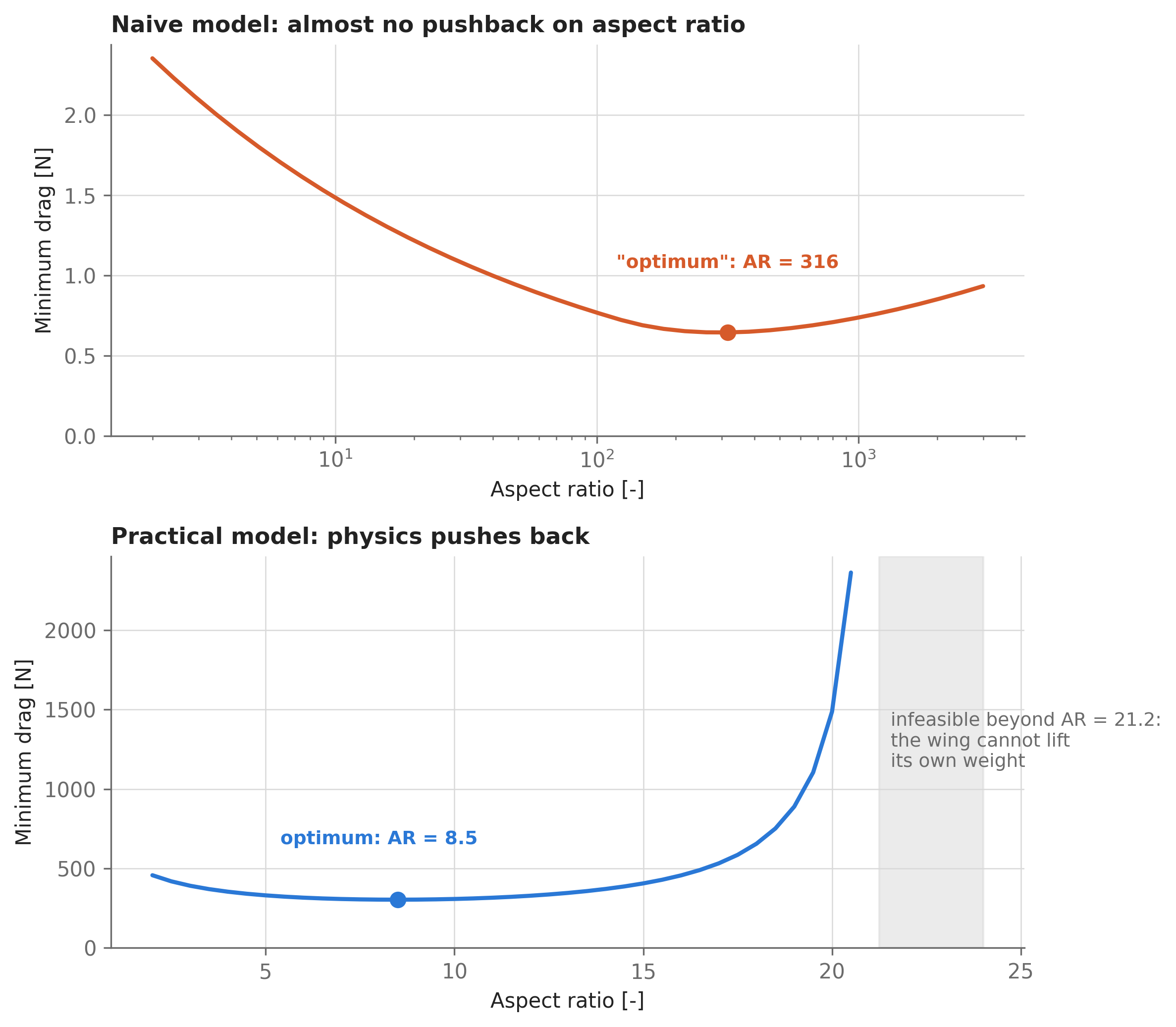
The two panels are the whole chapter in one picture. In the naive model, sweeping aspect ratio across three orders of magnitude changes the achievable drag by only a factor of 3.6 — the landscape is nearly flat, and its shallow minimum comes from a Reynolds-number effect that real designers would consider a rounding term. (The bowl is so flat that our coarse sweep grid bottoms out at \(AR =\) 316 while the free optimization found 296 — when the “optimum” moves that much between nearly identical problems, it isn’t an optimum so much as wherever the numerical dust happened to settle.) In the practical model, doubling the aspect ratio from its optimum costs 75% more drag (in the naive model, the same doubling costs 6%). And past \(AR \approx\) 21, the practical model doesn’t just discourage slenderness — it forbids it: the solver correctly reports the problem infeasible.
NoteWhy the feasibility cliff is exactly where it is
The takeoff constraint sets a minimum wing area proportional to weight: \(S \ge W / q_\mathrm{TO}\) with \(q_\mathrm{TO} = \tfrac{1}{2}\rho \, C_{L,\max} V_\mathrm{TO}^2\). Substituting that into the wing weight buildup makes wing weight scale linearly with gross weight, with a slope that grows as \(AR^{1.5}\). Weight closure then reads \(W \, (1 - k_1 - k_2 \, AR^{1.5}) \ge W_0\), which has a positive solution only while the parenthesis is positive — i.e., below \(AR_\mathrm{crit} = ((1 - k_1)/k_2)^{2/3} =\) 21.2, matching where the sweep’s solves start failing. Beyond it, every extra newton of wing demands more than one newton of additional lift capability: a structural death spiral. Infeasibility here isn’t a solver failure; it’s the model telling you the truth.
Summarizing the pushback (or lack of it) on each design freedom:
| Design freedom | Why the optimizer wants it | Pushback, naive model | Pushback, practical model |
|---|---|---|---|
| Raise aspect ratio | Induced drag falls as \(1/AR\) | Weak \(\mathrm{Re}\) penalty as the chord shrinks | Structural wing weight grows as \(AR^{1.5}\) |
| Shrink wing area | Less wetted area, less profile drag | None (until the \(C_L\) bound catches it) | Takeoff: must lift the airplane at 22 m/s at \(C_{L,\max}\) |
| Raise cruise \(C_L\) | Smaller, slower wing for the same lift | None — profile drag is blind to \(C_L\); rails against the hard bound | Induced drag grows as \(C_L^2\) |
| Change airspeed | — | None — a perfectly flat valley | Fuselage and profile drag grow as \(V^2\); induced drag grows as \(1/V^2\) |
This generalizes into a pre-flight checklist for any design optimization problem:
TipBefore you trust an optimum
- For every design variable, name the effect that punishes increasing it and the effect that punishes decreasing it. If either answer is “nothing,” expect that variable at a bound, at infinity, or wandering a flat valley — and don’t trust it.
- Treat variables pinned at hand-imposed bounds as bug reports. A bound doing the work of missing physics (like our \(C_L \le 1.2\)) yields designs that are artifacts of the bound, not the physics.
- Ask “why wouldn’t this work in real life?” Your answer names the missing model or constraint.
- Remember that optimization amplifies model error. A simulation with a modeling gap gives you a wrong number; an optimizer with a modeling gap actively seeks out the corner of the design space where the gap is largest, and parks your airplane there. The optimizer is a ruthless auditor of your models — your models must be able to push back.
10.6 Where to go next
- Chapter 11 scales this exact philosophy up to a full conceptual aircraft-sizing problem (SimPleAC): the same wing-weight and drag models, plus fuel burn via the Breguet range equation — and extraction of design sensitivities from the solution.
- Chapter 3 covers the craft of making models like these solver-friendly: log transforms, scaling, and keeping expressions NaN-free.
- Chapter 7 (and Chapter 6 for airfoils) shows how to replace the hand-rolled drag buildup used here with real, differentiable aerodynamics models — so that the physics pushing back on your optimizer is as trustworthy as possible.