13  The Dynamics Stack

The previous chapter (Section 12.1) taught trajectory optimization on toy systems, where writing out the equations of motion by hand took three lines. Real vehicles are messier: they fly in 3D, they have attitude and angular rates, and their forces arrive in a confusing mix of axis systems. This chapter introduces the AeroSandbox dynamics stack — a family of Dynamics classes that write the equations of motion for you, let you attach forces in whatever axis frame is most natural, and plug directly into Opti as differentiable constraints. You’ll learn to pick the right class for your problem’s fidelity level, then apply the stack to two showcase problems: a minimum-time quadcopter flip, and a maximum-range engine-out glide of a Cessna 152 with a real aerodynamics model in the loop. At the end, we show that the same classes work without an optimizer, as plain equation-of-motion calculators for scipy integration and flight-data visualization.

13.1 Why a dynamics engine?

The takeaway: you can write vehicle dynamics by hand as Opti constraints — and you should know how — but a dynamics engine removes the error-prone bookkeeping, and upgrades you to a more accurate integrator for free.

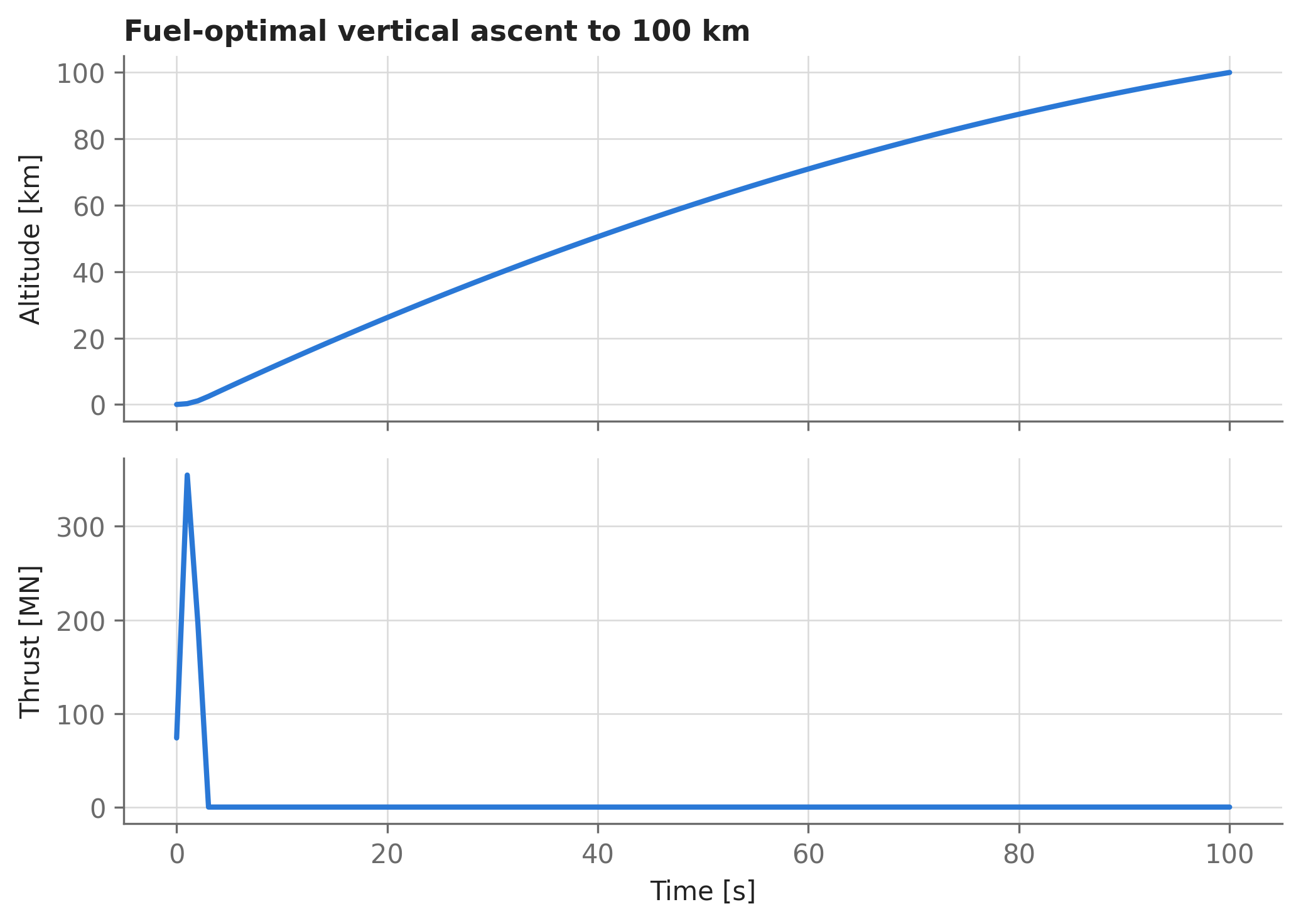
Let’s make that concrete with the simplest trajectory problem in this book: a rocket that must climb vertically to 100 km altitude in 100 seconds, burning as little fuel as possible. The physics is one force balance and one fuel-burn law: acceleration is thrust-over-mass minus gravity, and mass decreases in proportion to thrust (a constant specific impulse of 300 s).

13.1.1 By hand

Writing the dynamics manually means choosing a discretization and spelling it out. Here we use forward Euler — each state steps forward using the derivative at the start of the interval:

\[ \Delta z \approx v(t_1)\, \Delta t, \qquad \Delta v \approx \left(\frac{T(t_1)}{m(t_1)} - g\right) \Delta t, \qquad \Delta m \approx -\alpha\, T(t_1)\, \Delta t \]

import aerosandbox as asb
import aerosandbox.numpy as np

opti = asb.Opti()

N = 100  # number of discretization points
time = np.linspace(0, 100, N)  # sec

mass_initial = 500e3  # kg (a 500-metric-ton rocket)
z_final = 100e3  # m
g = 9.81  # m/s^2
alpha_fuel = 1 / (300 * g)  # kg of fuel per N-s of impulse (i.e., Isp = 300 s)

altitude = opti.variable(init_guess=np.linspace(0, z_final, N))
velocity = opti.variable(init_guess=z_final / 100, n_vars=N)
mass = opti.variable(init_guess=mass_initial, n_vars=N)
thrust = opti.variable(init_guess=g * mass_initial, n_vars=N, lower_bound=0)

opti.subject_to(
    [  # The dynamics, discretized manually with forward Euler:
        np.diff(altitude) == velocity[:-1] * np.diff(time),
        np.diff(velocity) == (thrust[:-1] / mass[:-1] - g) * np.diff(time),
        np.diff(mass) == -alpha_fuel * thrust[:-1] * np.diff(time),
    ]
)

opti.subject_to(
    [
        altitude[0] == 0,
        velocity[0] == 0,
        mass[0] == mass_initial,
        altitude[-1] == z_final,
        mass >= 0,
    ]
)

opti.minimize(-mass[-1])  # maximize final mass == minimize fuel burn

sol_manual = opti.solve(verbose=False)
fuel_manual = mass_initial - sol_manual(mass[-1])
print(f"Fuel burned (manual Euler, N={N}): {fuel_manual / 1e3:.1f} metric tons")

Fuel burned (manual Euler, N=100): 210.0 metric tons

This works, and for a 1D problem it’s perfectly reasonable. But notice what you had to get right by hand: the discretization scheme, the indexing ([:-1] everywhere), and the sign conventions. In 3D, with attitude dynamics, this approach balloons to hundreds of lines of quaternion or Euler-angle algebra — all of it an opportunity for silent sign errors.

13.1.2 With the dynamics engine

The same problem with asb.DynamicsPointMass1DVertical:

opti = asb.Opti()
time = np.linspace(0, 100, N)

dyn = asb.DynamicsPointMass1DVertical(
    mass_props=asb.MassProperties(
        mass=opti.variable(init_guess=mass_initial, n_vars=N)
    ),
    z_e=opti.variable(init_guess=np.linspace(0, -z_final, N)),
    w_e=opti.variable(init_guess=-z_final / 100, n_vars=N),
)

thrust = opti.variable(init_guess=g * mass_initial, n_vars=N, lower_bound=0)
dyn.add_force(Fz=-thrust)  # Earth axes are North-East-Down: "up" is -z!
dyn.add_gravity_force(g=g)

dyn.constrain_derivatives(opti, time)  # <-- the equations of motion, written for you

# Fuel burn isn't part of the standard point-mass state, so we add it ourselves:
opti.constrain_derivative(
    derivative=-alpha_fuel * thrust,
    variable=dyn.mass_props.mass,
    with_respect_to=time,
)

opti.subject_to(
    [
        dyn.z_e[0] == 0,
        dyn.w_e[0] == 0,
        dyn.mass_props.mass[0] == mass_initial,
        dyn.z_e[-1] == -z_final,
        dyn.mass_props.mass >= 0,
    ]
)

opti.minimize(-dyn.mass_props.mass[-1])

sol = opti.solve(verbose=False)
dyn = sol(dyn)  # substitutes optimized values into the Dynamics object, in-place

fuel_engine = mass_initial - dyn.mass_props.mass[-1]
print(f"Fuel burned (dynamics engine, N={N}): {fuel_engine / 1e3:.1f} metric tons")

Fuel burned (dynamics engine, N=100): 201.7 metric tons

The workflow, which every problem in this chapter repeats, is:

1. Instantiate a Dynamics class, passing Opti variables (or plain numbers) as the state variables.
2. Add forces with dyn.add_force() (and moments with dyn.add_moment(), for rigid-body classes), in whatever axis system each force is naturally expressed in. dyn.add_gravity_force() is a shorthand for the most common one.
3. dyn.constrain_derivatives(opti, time) — this computes the state derivatives from the accumulated forces and constrains the discretized trajectory to obey them, exactly like the opti.constrain_derivative() calls of Section 12.1, just applied to every state variable at once.
4. Add boundary conditions and an objective, solve, and call sol(dyn) to push the solved values back into the object for post-processing.

The optimal strategy is the classic one: burn hard early (while you’re heavy and every second spent hovering costs fuel), then cut the engine and coast to apogee.

13.1.3 Same physics, different answers?

Look closely at the two fuel burns: 210.0 tons by hand versus 201.7 tons with the engine — a 8.2-ton disagreement from the same physics on the same grid. The difference is the integrator: our manual version used forward Euler (first-order accurate), while constrain_derivatives() defaults to trapezoidal integration (second-order accurate), which averages the derivative across each interval. Refining the grid shows which one to believe:

def solve_rocket_trapezoidal(N_ref):
    opti = asb.Opti()
    time = np.linspace(0, 100, N_ref)
    z = opti.variable(init_guess=np.linspace(0, z_final, N_ref))
    v = opti.variable(init_guess=z_final / 100, n_vars=N_ref)
    m = opti.variable(init_guess=mass_initial, n_vars=N_ref)
    T = opti.variable(init_guess=g * mass_initial, n_vars=N_ref, lower_bound=0)
    opti.constrain_derivative(v, z, time)
    opti.constrain_derivative(T / m - g, v, time)
    opti.constrain_derivative(-alpha_fuel * T, m, time)
    opti.subject_to([z[0] == 0, v[0] == 0, m[0] == mass_initial, z[-1] == z_final, m >= 0])
    opti.minimize(-m[-1])
    return mass_initial - opti.solve(verbose=False)(m[-1])


fuel_ref = solve_rocket_trapezoidal(N_ref=2000)

err_manual = fuel_manual - fuel_ref
err_engine = fuel_engine - fuel_ref
print(f"Refined-grid reference fuel burn:  {fuel_ref / 1e3:.1f} tons")
print(f"Error, manual Euler at N={N}:      {err_manual / 1e3:+.1f} tons ({err_manual / fuel_ref:+.1%})")
print(f"Error, trapezoidal at N={N}:       {err_engine / 1e3:+.1f} tons ({err_engine / fuel_ref:+.1%})")

Refined-grid reference fuel burn:  199.0 tons
Error, manual Euler at N=100:      +10.9 tons (+5.5%)
Error, trapezoidal at N=100:       +2.7 tons (+1.3%)

At identical grid resolution, the trapezoidal answer lands roughly 4× closer to the refined-grid reference. That’s the “for free” part: the dynamics engine doesn’t just save typing, it defaults you into a better discretization. (For the systematic way to run refinement studies like this, see Section 12.1.)

13.2 The Dynamics family

The takeaway: pick the class whose state parameterization matches your problem — point-mass vs. rigid-body, 1D/2D/3D, Cartesian vs. speed-angle — and everything downstream (forces, frames, constraints) works identically.

Aerospace dynamics problems nearly all reduce to the same skeleton: a (roughly) rigid body moving through 3D space, sometimes simplified to 2D or 1D. Rather than one monolithic simulator, AeroSandbox provides a family of classes, each implementing the equations of motion for one combination of fidelity and state parameterization. The full 3D rigid-body class implements the standard nonlinear equations of motion (following Chapter 9 of Drela’s Flight Vehicle Aerodynamics); the others are progressively-reduced special cases. All of them share the interface you just saw: state, add_force(), constrain_derivatives(), state_derivatives().

Here is the whole family — this table is generated live from the library, so it always matches your installed version:

import pandas as pd

dynamics_classes = [
    asb.DynamicsPointMass1DHorizontal,
    asb.DynamicsPointMass1DVertical,
    asb.DynamicsPointMass2DCartesian,
    asb.DynamicsPointMass2DSpeedGamma,
    asb.DynamicsPointMass3DCartesian,
    asb.DynamicsPointMass3DSpeedGammaTrack,
    asb.DynamicsRigidBody2DBody,
    asb.DynamicsRigidBody3DBodyEuler,
]

table = pd.DataFrame(
    [
        {
            "Class": cls.__name__,
            "Model": "Rigid body" if "RigidBody" in cls.__name__ else "Point mass",
            "States": ", ".join(cls().state.keys()),
            "Controls": ", ".join(cls().control_variables.keys()),
        }
        for cls in dynamics_classes
    ]
)
table

	Class	Model	States	Controls
0	DynamicsPointMass1DHorizontal	Point mass	x_e, u_e	Fx_e
1	DynamicsPointMass1DVertical	Point mass	z_e, w_e	Fz_e
2	DynamicsPointMass2DCartesian	Point mass	x_e, z_e, u_e, w_e	alpha, Fx_e, Fz_e
3	DynamicsPointMass2DSpeedGamma	Point mass	x_e, z_e, speed, gamma	alpha, Fx_w, Fz_w
4	DynamicsPointMass3DCartesian	Point mass	x_e, y_e, z_e, u_e, v_e, w_e	alpha, beta, bank, Fx_e, Fy_e, Fz_e
5	DynamicsPointMass3DSpeedGammaTrack	Point mass	x_e, y_e, z_e, speed, gamma, track	alpha, beta, bank, Fx_w, Fy_w, Fz_w
6	DynamicsRigidBody2DBody	Rigid body	x_e, z_e, u_b, w_b, theta, q	Fx_b, Fz_b, My_b
7	DynamicsRigidBody3DBodyEuler	Rigid body	x_e, y_e, z_e, u_b, v_b, w_b, phi, theta, psi,...	Fx_b, Fy_b, Fz_b, Mx_b, My_b, Mz_b, hx_b, hy_b...

Reading the names: DynamicsPointMass2DSpeedGamma is a point mass, in 2D, with velocity parameterized as speed and flight-path angle (\(V\), \(\gamma\)) rather than Cartesian components. The “Controls” column lists both true control inputs (forces \(F\), moments \(M\)) and indirect controls like alpha — quantities that aren’t states (they have no time derivative in the model) but that you’ll typically make decision variables so the optimizer can steer with them.

The mass_props argument accepts an asb.MassProperties object (mass, CG location, and — for the rigid-body classes — the full inertia tensor; see Section 5.7). Point-mass classes only use the mass; rigid-body classes use everything.

13.2.1 Three axis systems

Every force on an aircraft is most naturally expressed in some frame: gravity acts straight down, thrust acts along the airframe, and lift and drag are defined relative to the incoming wind. The dynamics stack lets you state each force in its natural frame and handles all rotations internally. The three frames you’ll use constantly:

• Earth axes ("earth"): fixed to the ground, using the North-East-Down (NED) convention. This trips up everyone at least once: \(z_e\) points down, so altitude is \(-z_e\) (every Dynamics class provides dyn.altitude so you never have to remember). NED assumes a locally-flat Earth.
• Body axes ("body"): painted onto the vehicle. \(x_b\) points forward out the nose, \(y_b\) out the right wing, \(z_b\) down through the belly.
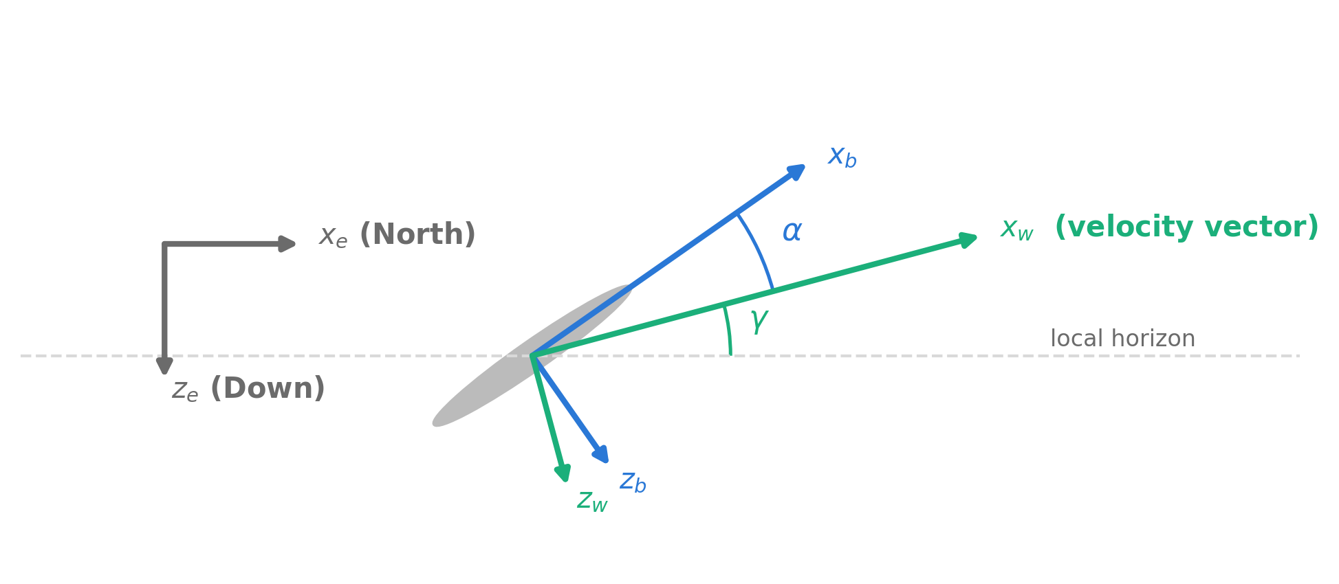
• Wind axes ("wind"): aligned with the velocity vector. \(x_w\) points into the relative wind (i.e., along the direction of flight), \(z_w\) points downward perpendicular to it. Drag is therefore a force in the \(-x_w\) direction, and lift is in the \(-z_w\) direction — both negated, another classic sign trap.

Figure 13.1: The three axis systems of the dynamics stack, in a 2D side view. Pitch angle θ orients the body frame, flight-path angle γ orients the wind frame (which follows the velocity vector), and angle of attack α = θ − γ separates them. Note that all three z-axes point generally downward — Earth axes are North-East-Down.

Two methods put these frames to work:

• dyn.add_force(Fx=..., Fy=..., Fz=..., axes="wind") accumulates a force expressed in any frame (same for add_moment on rigid-body classes). You saw axes="earth" implicitly in add_gravity_force().
• dyn.convert_axes(x, y, z, from_axes="body", to_axes="earth") converts any vector between frames, using the instance’s current attitude. (Two more frames, "geometry" and "stability", exist for interfacing with geometry and aerodynamics tools.)

Finally, every Dynamics instance exposes dyn.op_point: an asb.OperatingPoint built from the current state, complete with an Atmosphere evaluated at the instance’s altitude (see Section 9.2). This one property is the bridge between dynamics and aerodynamics — you can hand it straight to an aero model, as we’ll do in the Cessna case below.

13.2.2 Choosing a fidelity level

Which class should you use? Match the timescales:

• Maneuver problems (seconds): if the vehicle’s rotational dynamics matter — a quadcopter flip, a fighter pull-up, spin recovery — use a rigid-body class. You get attitude (\(\phi, \theta, \psi\)) and angular rates (\(p, q, r\)) as states, driven by moments through the full inertia tensor.
• Mission and performance problems (minutes to hours): an airplane’s short-period and lateral modes settle in seconds, far faster than the energy management you care about. A point-mass class discards them: angular rates are assumed zero, and attitude becomes a control you prescribe (via alpha, bank) rather than a state you integrate. For longitudinal problems, DynamicsPointMass2DSpeedGamma — states \(x_e, z_e, V, \gamma\) — is the workhorse; its 3D sibling DynamicsPointMass3DSpeedGammaTrack adds a heading (“track”) state and a bank-angle control for problems like engine-out turnbacks.

This is the same physical judgment as choosing between an Euler code and a panel method in aerodynamics: not “which model is best,” but “which model is the cheapest one that resolves the physics my decision depends on.”

13.3 Case study 1: a minimum-time quadcopter flip

The takeaway: with a rigid-body dynamics class, a genuinely aggressive optimal-control problem — a full 360° flip — is about 40 lines of code.

Consider an idealized 2D quadcopter: a 0.1 kg bar, 0.1 m wide, with one rotor at each end. Each rotor produces 0 to 1 N of thrust along the body \(-z_b\) axis (i.e., “up” when the vehicle is level), so the vehicle has a thrust-to-weight ratio of about 2. Equal thrusts accelerate it; differential thrust creates a pitching moment about the center — that’s the only way it can rotate.

First, a drawing helper so we can see what the vehicle is doing (matplotlib patches; nothing AeroSandbox-specific — feel free to skip):

import _common
import matplotlib as mpl
import matplotlib.pyplot as plt

# Single-hue sequential colormap for thrust magnitude (light = low, dark = high):
thrust_cmap = mpl.colors.LinearSegmentedColormap.from_list(
    "thrust", ["#d6e5f7", "#0b3c74"]
)
thrust_norm = mpl.colors.Normalize(vmin=0, vmax=1)


def draw_quad_trajectory(
    dyn, left_thrust, right_thrust, interval=5, magnify=1.0, figsize=(8, 4.5)
):
    """Draws the quadcopter every `interval`-th timestep along its trajectory,
    with rotors colored by their instantaneous thrust."""
    fig, ax = plt.subplots(figsize=figsize)
    ax.plot(dyn.x_e, -dyn.z_e, color=_common.GRID, lw=1.5, zorder=1)  # path

    for i in range(0, len(dyn), interval):
        d = dyn[i]  # Dynamics instances are indexable: one snapshot in time
        xform = (
            mpl.transforms.Affine2D()
            .scale(0.1 * magnify)  # vehicle is 0.1 m wide
            .rotate(d.theta)
            .translate(d.x_e, -d.z_e)
            + ax.transData
        )
        patches = [
            mpl.patches.Rectangle((-0.5, -0.06), 1.0, 0.12, color=_common.TEXT_PRIMARY),
            mpl.patches.Ellipse(
                (-0.5, 0.16), 0.62, 0.17, color=thrust_cmap(thrust_norm(left_thrust[i]))
            ),
            mpl.patches.Ellipse(
                (0.5, 0.16), 0.62, 0.17, color=thrust_cmap(thrust_norm(right_thrust[i]))
            ),
        ]
        for patch in patches:
            patch.set_transform(xform)
            patch.set_zorder(5)
            ax.add_patch(patch)

    fig.colorbar(
        mpl.cm.ScalarMappable(norm=thrust_norm, cmap=thrust_cmap),
        ax=ax, label="Rotor thrust [N]", shrink=0.85,
    )
    ax.set_aspect("equal", adjustable="box")
    ax.set_xlabel("$x_e$ [m]")
    ax.set_ylabel("Altitude $-z_e$ [m]")
    if magnify != 1:
        ax.annotate(
            f"Vehicle drawn {magnify:g}× larger for visibility.",
            xy=(0.5, 0.02), xycoords="axes fraction", ha="center", fontsize=8,
            color=_common.TEXT_SECONDARY,
        )
    return fig, ax


quad_mass_props = asb.MassProperties(
    mass=0.1,  # kg
    Iyy=0.5 * 0.1 * 0.1**2,  # pitch inertia [kg·m²]; Ixx/Izz don't matter in 2D
    Ixx=1, Izz=1,
)

13.3.1 Simulation is just optimization with nothing left to choose

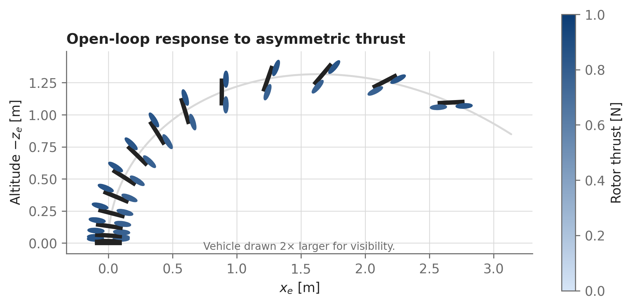
Before optimizing anything, note a useful degenerate case: if you prescribe all the control inputs and the initial state, the “optimization problem” has exactly as many constraints as unknowns — there are no degrees of freedom left, and no objective is needed. opti.solve() then simply integrates the trajectory (it solves the discretized equations of motion as a root-finding problem — the same trick as the feasibility problems of Section 5.6). Here’s one second of flight with slightly asymmetric rotor thrusts:

opti = asb.Opti()

N = 150
time = np.linspace(0, 1, N)  # sec

left_thrust = 0.85 * np.ones(N)  # N (prescribed, not a variable!)
right_thrust = 0.78 * np.ones(N)

dyn = asb.DynamicsRigidBody2DBody(
    mass_props=quad_mass_props,
    x_e=opti.variable(init_guess=0, n_vars=N),
    z_e=opti.variable(init_guess=0, n_vars=N),
    u_b=opti.variable(init_guess=0, n_vars=N),
    w_b=opti.variable(init_guess=0, n_vars=N),
    theta=opti.variable(init_guess=0, n_vars=N),
    q=opti.variable(init_guess=0, n_vars=N),
)

dyn.add_force(Fz=-(left_thrust + right_thrust), axes="body")  # rotors push "up"
dyn.add_moment(My=(right_thrust - left_thrust) * 0.1 / 2)  # differential thrust
dyn.add_gravity_force()

dyn.constrain_derivatives(opti, time)

opti.subject_to(  # initial condition: at rest at the origin
    [dyn.x_e[0] == 0, dyn.z_e[0] == 0, dyn.u_b[0] == 0,
     dyn.w_b[0] == 0, dyn.theta[0] == 0, dyn.q[0] == 0]
)

sol = opti.solve(verbose=False)  # no objective: this is pure simulation
dyn = sol(dyn)

Figure 13.2: One second of open-loop flight with mismatched rotor thrusts (left 0.85 N, right 0.78 N). Thrust above weight lofts the vehicle at first, but the imbalance steadily torques it over; once tipped, the thrust vector swings sideways and the quad careens off downrange — anyone’s first flight on a real quadcopter.

13.3.2 Now, the flip

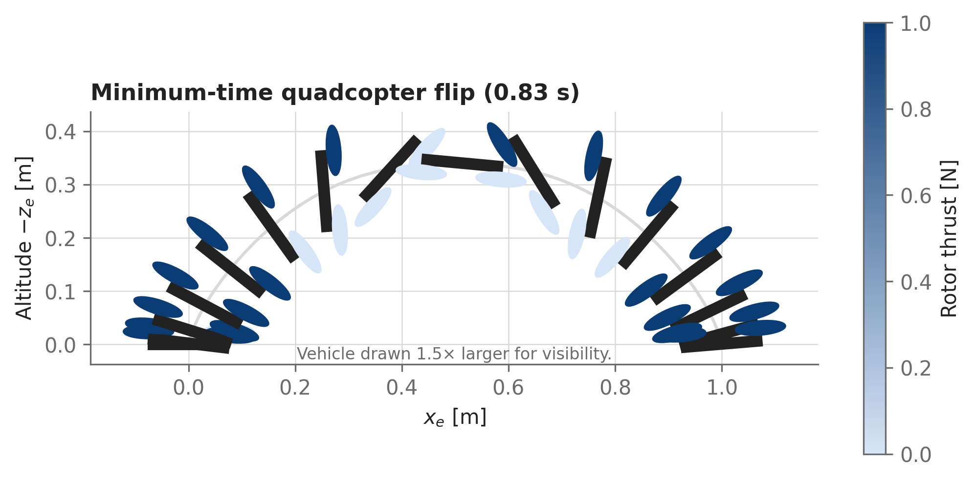
Time to fly it properly. The mission: start at rest at the origin, end at rest 1 m to the right, having completed one full 360° pitch flip on the way — in minimum time. Both rotor thrusts become decision variables (bounded 0–1 N), and so does the final time itself (a free-final-time problem, exactly as in Section 12.1):

opti = asb.Opti()

N = 80
time_final = opti.variable(init_guess=1, lower_bound=0)
time = np.linspace(0, time_final, N)

left_thrust = opti.variable(init_guess=0.7, n_vars=N, lower_bound=0, upper_bound=1)
right_thrust = opti.variable(init_guess=0.6, n_vars=N, lower_bound=0, upper_bound=1)

dyn = asb.DynamicsRigidBody2DBody(
    mass_props=quad_mass_props,
    x_e=opti.variable(init_guess=np.linspace(0, 1, N)),
    z_e=opti.variable(init_guess=0, n_vars=N),
    u_b=opti.variable(init_guess=0, n_vars=N),
    w_b=opti.variable(init_guess=0, n_vars=N),
    theta=opti.variable(init_guess=np.linspace(0, -2 * np.pi, N)),
    q=opti.variable(init_guess=0, n_vars=N),
)

dyn.add_force(Fz=-(left_thrust + right_thrust), axes="body")
dyn.add_moment(My=(right_thrust - left_thrust) * 0.1 / 2)
dyn.add_gravity_force()

dyn.constrain_derivatives(opti, time)

opti.subject_to(  # start: at rest at the origin
    [dyn.x_e[0] == 0, dyn.z_e[0] == 0, dyn.u_b[0] == 0,
     dyn.w_b[0] == 0, dyn.theta[0] == 0, dyn.q[0] == 0]
)
opti.subject_to(  # end: at rest at (1, 0), having flipped through -360°
    [dyn.x_e[-1] == 1, dyn.z_e[-1] == 0, dyn.u_b[-1] == 0,
     dyn.w_b[-1] == 0, dyn.theta[-1] == np.radians(-360), dyn.q[-1] == 0]
)

opti.minimize(time_final)

sol = opti.solve(verbose=False)
dyn = sol(dyn)
flip_time = sol(time_final)
print(f"Minimum-time flip completed in {flip_time:.3f} sec.")

Minimum-time flip completed in 0.826 sec.

Note the initial guess for theta: np.linspace(0, -2 * np.pi, N) sketches “rotate once, nose-forward” for the optimizer. Free-final-time flip problems are nonconvex — guess +2π instead and you’ll converge to an equally-valid backflip. Providing a rough storyboard of the maneuver as the initial guess is standard practice (see Section 12.1).

Figure 13.3: The minimum-time flip. The quadcopter leaps up and to the right, commits to the rotation, completes most of the flip near the top of its hop, and catches itself at the far boundary condition.

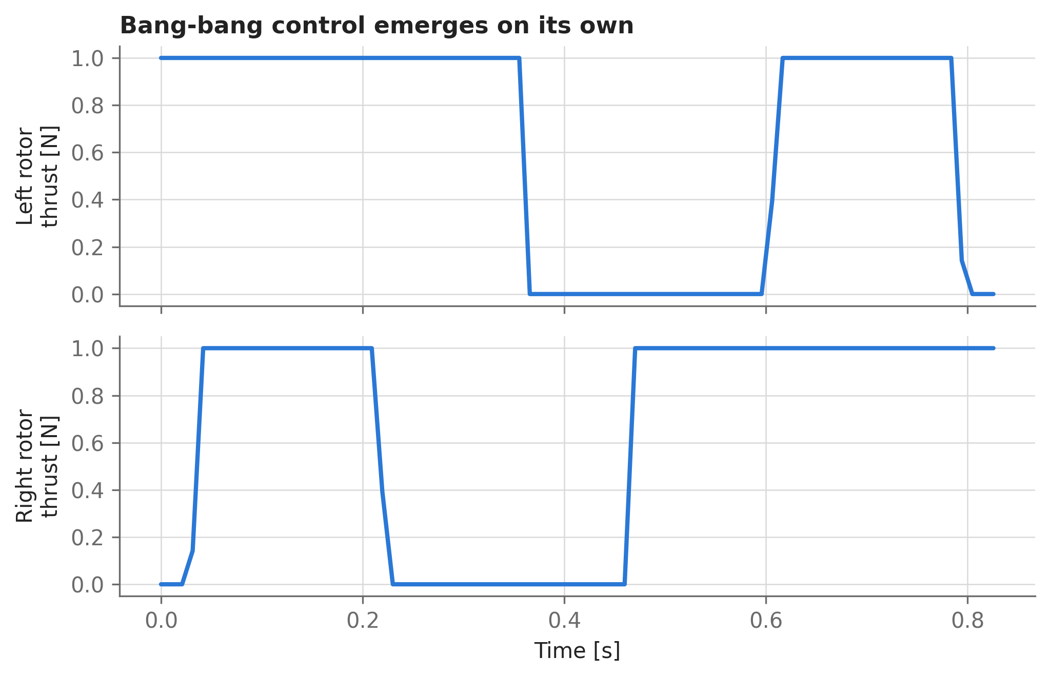
Figure 13.4: Rotor thrust histories for the flip. The solution is essentially bang-bang: each rotor slams between its bounds, and the two commands mirror each other to torque the vehicle into, and then out of, the rotation.

Nobody told the optimizer to use bang-bang control — it discovered that saturating the actuators is time-optimal, which is exactly what optimal-control theory predicts for this class of problem. This entire study is roughly 40 lines of model code, and it solves in seconds.

13.4 Case study 2: engine-out glide of a Cessna 152

The takeaway: dyn.op_point lets you drop a full physics-based aerodynamics model into the trajectory optimization loop — the optimizer then rediscovers, on its own, what flight instructors teach about engine-out glides.

Picture a Cessna 152 cruising at 107 knots, 1000 m above central Massachusetts, when the engine sputters and dies. Two questions matter immediately: how far can it glide, and how should the pilot fly to achieve that? This is a mission-performance problem — minutes long, no aerobatics — so per Section 13.2.2 we use the 2D point-mass class with speed–flight-path-angle states, and the angle of attack becomes the pilot’s control input.

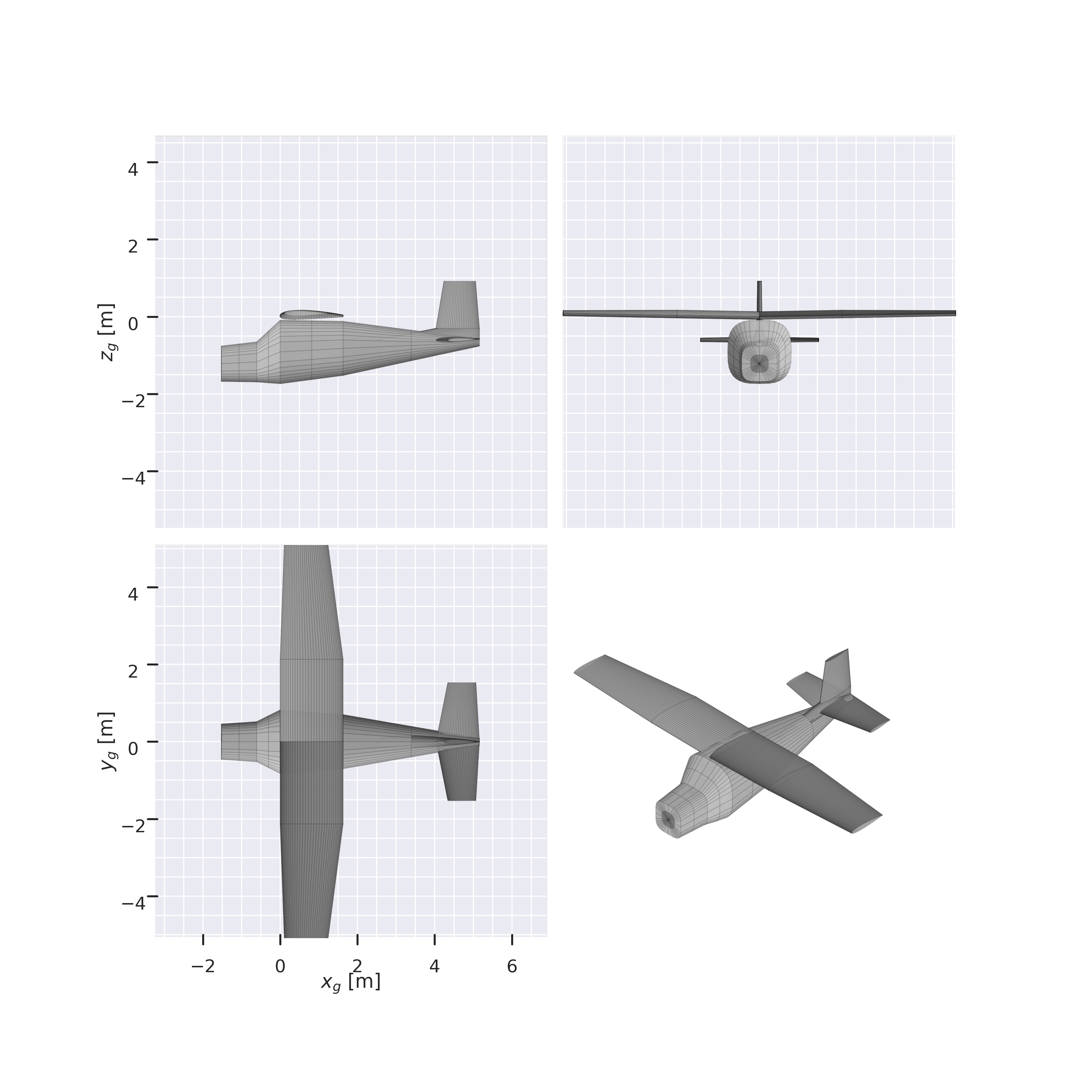
Unlike the quadcopter (whose “aerodynamics” was two thrust numbers), this problem needs a real force model. We define the airplane’s geometry with asb.Airplane (the subject of Section 5.1 — the details are collapsed below) and let asb.AeroBuildup (Section 7.3) predict its lift and drag.

import aerosandbox as asb
import aerosandbox.numpy as np
from aerosandbox.tools import units as u


def ft(feet, inches=0.0):  # converts feet (and inches) to meters
    return feet * u.foot + inches * u.inch


airplane = asb.Airplane(
    name="Cessna 152",
    wings=[
        asb.Wing(
            name="Wing",
            xsecs=[
                asb.WingXSec(
                    xyz_le=[0, 0, 0], chord=ft(5, 4), airfoil=asb.Airfoil("naca2412")
                ),
                asb.WingXSec(
                    xyz_le=[0, ft(7), ft(7) * np.sind(1)],
                    chord=ft(5, 4),
                    airfoil=asb.Airfoil("naca2412"),
                ),
                asb.WingXSec(
                    xyz_le=[
                        ft(4, 3 / 4) - ft(3, 8 + 1 / 2),
                        ft(33, 4) / 2,
                        ft(33, 4) / 2 * np.sind(1),
                    ],
                    chord=ft(3, 8 + 1 / 2),
                    airfoil=asb.Airfoil("naca0012"),
                ),
            ],
            symmetric=True,
        ),
        asb.Wing(
            name="Horizontal Stabilizer",
            xsecs=[
                asb.WingXSec(
                    xyz_le=[0, 0, 0],
                    chord=ft(3, 8),
                    airfoil=asb.Airfoil("naca0012"),
                    twist=-2,
                ),
                asb.WingXSec(
                    xyz_le=[ft(1), ft(10) / 2, 0],
                    chord=ft(2, 4 + 3 / 8),
                    airfoil=asb.Airfoil("naca0012"),
                    twist=-2,
                ),
            ],
            symmetric=True,
        ).translate([ft(13, 3), 0, ft(-2)]),
        asb.Wing(
            name="Vertical Stabilizer",
            xsecs=[
                asb.WingXSec(
                    xyz_le=[ft(-5), 0, 0],
                    chord=ft(8, 8),
                    airfoil=asb.Airfoil("naca0012"),
                ),
                asb.WingXSec(
                    xyz_le=[ft(0), 0, ft(1)],
                    chord=ft(3, 8),
                    airfoil=asb.Airfoil("naca0012"),
                ),
                asb.WingXSec(
                    xyz_le=[ft(0, 8), 0, ft(5)],
                    chord=ft(2, 8),
                    airfoil=asb.Airfoil("naca0012"),
                ),
            ],
        ).translate([ft(16, 11) - ft(3, 8), 0, ft(-2)]),
    ],
    fuselages=[
        asb.Fuselage(
            xsecs=[
                asb.FuselageXSec(xyz_c=[0, 0, ft(-1)], radius=0),
                asb.FuselageXSec(xyz_c=[0, 0, ft(-1)], radius=ft(1.5), shape=4),
                asb.FuselageXSec(xyz_c=[ft(3), 0, ft(-0.85)], radius=ft(1.7), shape=4),
                asb.FuselageXSec(xyz_c=[ft(5), 0, ft(0)], radius=ft(2.7), shape=3),
                asb.FuselageXSec(xyz_c=[ft(10, 4), 0, ft(0.3)], radius=ft(2.3), shape=3),
                asb.FuselageXSec(xyz_c=[ft(21, 11), 0, ft(0.8)], radius=ft(0.3)),
            ]
        )
        .translate([ft(-5), 0, ft(-3)])
        .subdivide_sections(2)
    ],
)

airplane.draw_three_view()

array([[<Axes3D: zlabel='$z_g$ [m]'>, <Axes3D: >],
       [<Axes3D: xlabel='$x_g$ [m]', ylabel='$y_g$ [m]'>, <Axes3D: >]],
      dtype=object)

<module '_common' from '/tmp/claude-1000/-home-psharpe-gh-AeroSandbox/1ccf6b40-3256-4f8d-9484-ebe00c7e55db/scratchpad/book-staging/_common.py'>

13.4.1 How well does it glide?

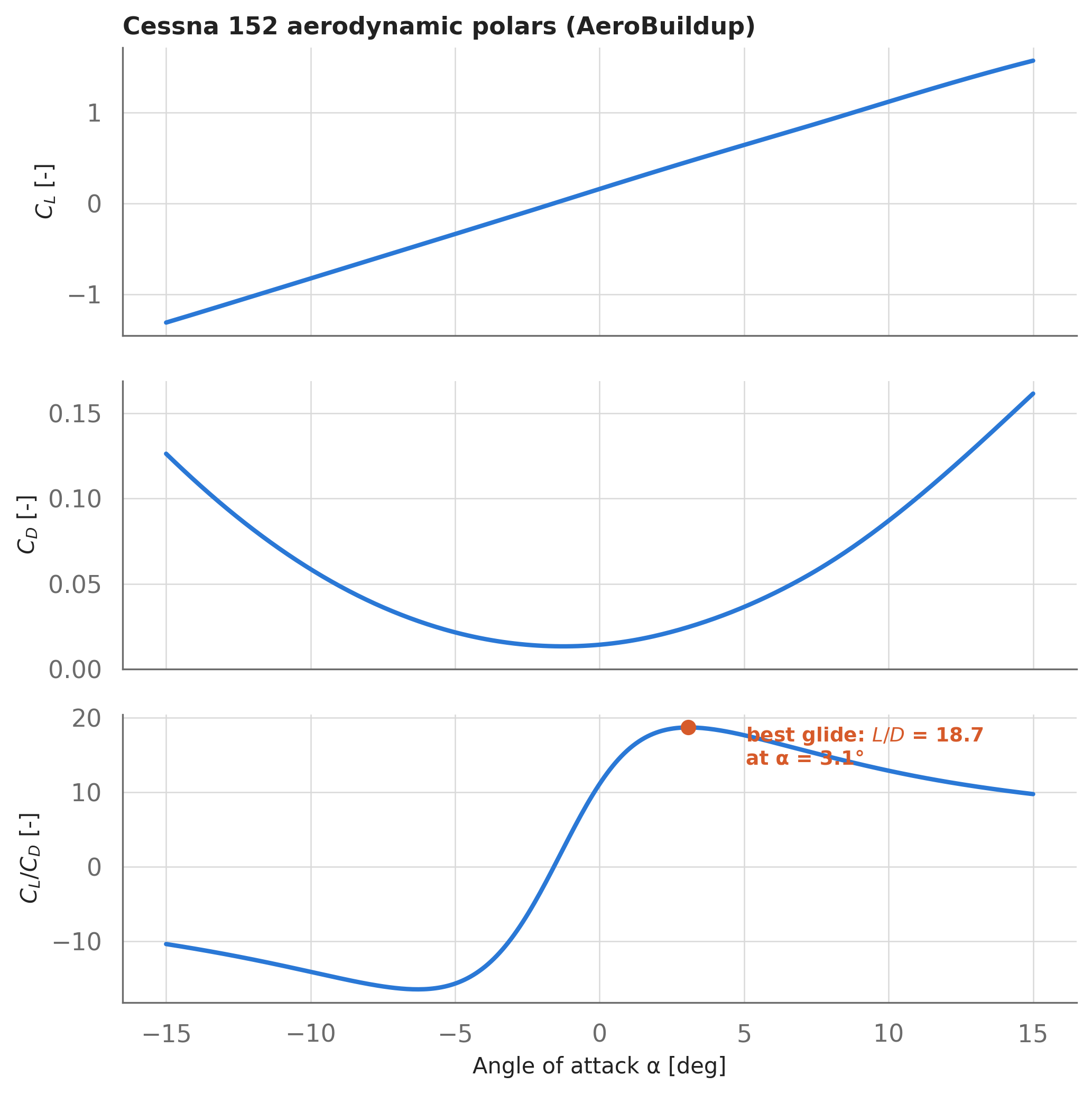
Before optimizing a trajectory, sanity-check the aerodynamics with a quick polar sweep. AeroBuildup is fully vectorized, so all 300 angles of attack evaluate in one call:

alpha_sweep = np.linspace(-15, 15, 300)  # deg
aero_sweep = asb.AeroBuildup(
    airplane=airplane,
    op_point=asb.OperatingPoint(velocity=107 * u.knot, alpha=alpha_sweep),
).run()

LD = aero_sweep["CL"] / aero_sweep["CD"]
LD_max = np.max(LD)
alpha_LD_max = alpha_sweep[np.argmax(LD)]
print(f"Predicted best glide ratio: {LD_max:.1f}, at alpha = {alpha_LD_max:.1f} deg")

Predicted best glide ratio: 18.7, at alpha = 3.1 deg

Figure 13.5: AeroBuildup polars for the Cessna 152 model at 107 knots. Lift is linear until stall onset; drag grows quadratically away from its minimum; and their ratio peaks at the best-glide angle of attack (marked).

WarningTrust, but calibrate

AeroBuildup predicts a best glide ratio of 18.7; the FAA quotes roughly 9:1 for a real, engine-out Cessna 152. The model isn’t broken — our inputs are idealized. A stopped, non-feathering propeller is a large drag brake; we omitted the landing gear, wing struts, cooling-air momentum losses, antennas, rivets, and control-surface gaps. Per Hoerner’s Fluid-Dynamic Drag, such “everything else” items can roughly double a light aircraft’s profile drag. The lesson generalizes: a clean-geometry aero model gives you the clean-geometry answer, and closing the gap to flight data is a drag-accounting exercise, not a solver problem. For this study the shape of the optimal trajectory is unaffected; just mentally halve the range numbers.

13.4.2 The trajectory problem

Now the optimization: maximize final downrange distance \(x_e\), starting from 1000 m altitude at cruise speed. The final time is free (we let the optimizer stretch the time grid via a log_transformed variable, since durations are strictly positive — see Section 3.4). The one genuinely new line is passing dyn.op_point — a symbolic operating point, containing the optimizer’s current guesses of speed, altitude, and angle of attack at all 50 time nodes — directly into AeroBuildup. The entire aerodynamics model is thereby traced into the optimization graph, derivatives and all.

from time import perf_counter

opti = asb.Opti()

### Time discretization: free final time, cosine-spaced to resolve both ends
N = 50
time = np.cosspace(0, opti.variable(init_guess=180, log_transform=True), N)
time_guess = np.linspace(0, 180, N)

### Mass properties (a 152 near max gross, solo pilot)
mass_props = asb.mass_properties_from_radius_of_gyration(
    mass=1151.8 * u.lbm,
    radius_of_gyration_x=2, radius_of_gyration_y=3, radius_of_gyration_z=3,  # m
)

### Initial state
init_state = {
    "x_e": 0,
    "z_e": -1000,  # 1000 m altitude (remember: Earth-axes z points down)
    "speed": 107 * u.knot,  # cruise speed at the moment of engine failure
    "gamma": 0,
}

dyn = asb.DynamicsPointMass2DSpeedGamma(
    mass_props=mass_props,
    x_e=opti.variable(init_guess=init_state["speed"] * time_guess),
    z_e=opti.variable(init_guess=np.linspace(init_state["z_e"], 0, N)),
    speed=opti.variable(init_guess=init_state["speed"], n_vars=N),
    gamma=opti.variable(init_guess=0, n_vars=N,
                        lower_bound=-np.pi / 2, upper_bound=np.pi / 2),
    alpha=opti.variable(init_guess=5, n_vars=N,  # the control input [deg]
                        lower_bound=-5, upper_bound=15),
)
for k in dyn.state.keys():
    opti.subject_to(dyn.state[k][0] == init_state[k])

### Forces: gravity, plus the full AeroBuildup model evaluated on the trajectory
dyn.add_gravity_force(g=9.81)

aero = asb.AeroBuildup(airplane=airplane, op_point=dyn.op_point).run()
dyn.add_force(*aero["F_w"], axes="wind")  # aero forces, in wind axes

### Stay above ground, obey the equations of motion, and glide far
opti.subject_to(dyn.altitude > 0)
dyn.constrain_derivatives(opti, time)
opti.minimize(-dyn.x_e[-1])

t_start = perf_counter()
sol = opti.solve(verbose=False)
dyn = sol(dyn)
t_solve = perf_counter() - t_start

glide_range = dyn.x_e[-1]
glide_time = sol(time)[-1]
print(f"Solved in {sol.stats()['iter_count']} iterations ({t_solve:.0f} s).")
print(f"Maximum glide range: {glide_range / 1e3:.1f} km, reached in {glide_time / 60:.1f} min.")

Solved in 26 iterations (73 s).
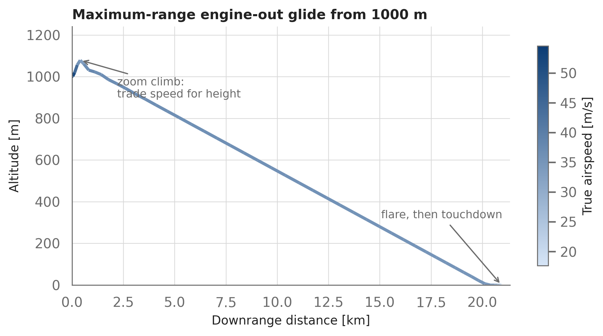
Maximum glide range: 20.9 km, reached in 9.8 min.

Figure 13.6: The maximum-range glide, colored by true airspeed. The airplane first zoom-climbs — trading its excess cruise speed for altitude — then settles onto a steady best-glide descent, and finally flares in the last seconds to squeeze out the remaining kinetic energy. Note the extreme aspect-ratio distortion: the descent is actually a shallow ~3° slope.

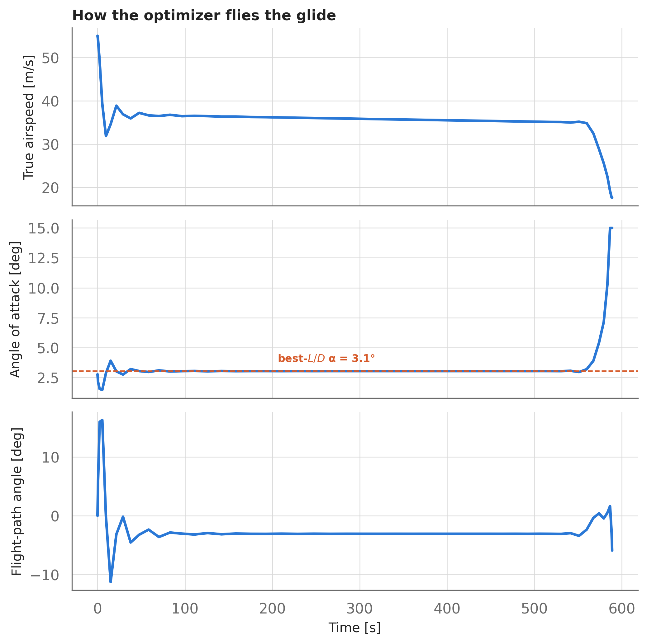
Figure 13.7: State and control histories for the optimal glide. Speed bleeds from 55 m/s cruise down to best-glide speed and holds (with a lightly-damped phugoid-like transient at the start); angle of attack sits on the best-L/D value for nearly the entire descent, then ramps to its limit in the final flare; the flight-path angle shows the initial zoom climb, the long shallow descent, and the flare.

13.4.3 What the optimizer figured out

The solution reads like a flight-training syllabus:

1. Pitch up immediately. Cruise speed (55 m/s) is far above best-glide speed; holding it would just burn energy into drag. The optimizer converts the excess kinetic energy into ~79 m of extra altitude — a zoom climb. This is precisely the “pitch for best glide” reflex that instructors drill.
2. Hold best glide. For the long middle portion, the commanded angle of attack (median 3.0°) sits essentially on the best-\(L/D\) value of 3.1° from our polar sweep — the dashed line in the middle panel above — at a steady 36 m/s. The slow decay in true airspeed during the descent isn’t the pilot slowing down; it’s the air getting denser on the way down at nearly-constant indicated airspeed.
3. Flare at the end. In the last seconds, the optimizer pulls to the α limit, spending the remaining kinetic energy to stretch the glide a final few hundred meters. (A real pilot should keep an energy reserve for obstacles — the optimizer, told that the world ends at touchdown, does not.)

An energy audit confirms the physics. The airplane starts with an energy height (altitude plus kinetic energy expressed as height, \(h + V^2/2g\)) of 1154 m; multiplying by the best glide ratio of 18.7 bounds the achievable range at 21.6 km. The optimized trajectory achieves 20.9 km — 97% of that ideal, with the shortfall being drag paid during off-best-glide segments (the zoom climb and flare).

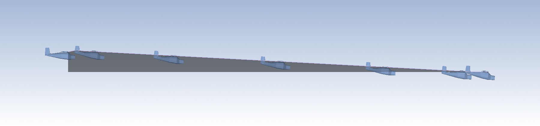
For a qualitative look at the whole trajectory, every Dynamics instance has a draw() method that renders the vehicle along its path in 3D (using PyVista), complete with an altitude drape and ground plane:

import pyvista as pv

pv.OFF_SCREEN = True  # render headless (no interactive window) for this book

plotter = dyn.draw(
    vehicle_model=airplane,
    show=False,
    n_vehicles_to_draw=7,
    draw_global_grid=False,  # grid + axes get cluttered at this 20:1 aspect ratio
    draw_global_axes=False,
    draw_axes=False,
)
plotter.window_size = (1800, 420)
plotter.camera.enable_parallel_projection()  # 2D-ify the view
plotter.camera_position = "xz"
plotter.camera.roll = 180  # NED axes: rotate so that "up" is up
plotter.camera.azimuth = 180
plotter.camera.zoom(3.6)
plotter.screenshot("glide_3d.png")
plotter.close()

from IPython.display import Image

Image("glide_3d.png")

Figure 13.8: The glide trajectory rendered by dyn.draw(), viewed side-on: the airplane model is drawn at intervals along the path (auto-scaled for visibility), with a gray drape below it indicating height above the ground. The nose-high flare at far right is clearly visible.

The same modeling pattern — point-mass dynamics plus AeroBuildup forces — extends directly to 3D with DynamicsPointMass3DSpeedGammaTrack, which adds heading and bank: that’s the setup for engine-out turnback studies (“the impossible turn”), terrain-following racing lines, and community-noise-optimal departure paths.

13.5 Dynamics without an optimizer

The takeaway: the Dynamics classes are equation-of-motion calculators first and Opti citizens second — you can drive them with any ODE integrator, or with no integrator at all.

Everything above embedded the dynamics in an optimization problem. But sometimes you just want to simulate: no decisions, no objective, possibly stiff dynamics where an adaptive off-the-shelf integrator shines. Three methods make any Dynamics class a drop-in right-hand side for scipy.integrate.solve_ivp:

• dyn.state_derivatives() — returns \(d(\text{state})/dt\) as a dict, given the instance’s current state and accumulated forces;
• dyn.pack_state() / dyn.unpack_state() — convert between that dict representation and the flat arrays scipy expects.

Here’s a worked example with genuinely nasty (near-singular) dynamics. It’s your birthday; someone hands you a helium balloon — a 5-gram rubber sphere, 10 inches in diameter at sea level — and at the end of the day, you let it go. Where does it end up? Assume (unrealistically, as we’ll see) that the balloon stretches freely so its internal pressure tracks ambient.

from scipy import integrate
from aerosandbox.atmosphere.atmosphere import gas_constant_universal

### Balloon parameters
mass_rubber = 0.005  # kg
helium_molar_mass = 4.002602e-3  # kg/mol
atmo_sl = asb.Atmosphere(altitude=0)
volume_sl = 4 / 3 * np.pi * ((10 * u.inch) / 2) ** 3
mass_helium = (  # PV = nRT
    atmo_sl.pressure() * volume_sl * helium_molar_mass
    / (gas_constant_universal * atmo_sl.temperature())
)

dyn_template = asb.DynamicsPointMass2DCartesian(
    mass_props=asb.MassProperties(mass=mass_rubber + mass_helium)
)


def balloon_volume(atmosphere):  # balloon stretches so P_inside tracks P_ambient
    return (
        mass_helium / helium_molar_mass * gas_constant_universal
        * atmosphere.temperature() / atmosphere.pressure()
    )


def equations_of_motion(t, y):
    g = 9.81
    dyn = dyn_template.get_new_instance_with_state(dyn_template.pack_state(y))
    dyn.add_gravity_force(g=g)

    # Buoyancy: weight of displaced air, pointing up (-z in Earth axes)
    volume = balloon_volume(dyn.op_point.atmosphere)
    dyn.add_force(Fz=-volume * dyn.op_point.atmosphere.density() * g, axes="earth")

    # Drag on a sphere (CD ~ 0.4 across the relevant Reynolds range)
    radius = (volume * 3 / (4 * np.pi)) ** (1 / 3)
    dyn.add_force(
        Fx=-dyn.op_point.dynamic_pressure() * 0.4 * np.pi * radius**2, axes="wind"
    )

    return dyn.unpack_state(dyn.state_derivatives())


t_eval = np.cosspace(0, 6 * 3600, 300)  # six hours
res = integrate.solve_ivp(
    fun=equations_of_motion,
    t_span=(t_eval.min(), t_eval.max()),
    t_eval=t_eval,
    y0=dyn_template.unpack_state({"x_e": 0, "z_e": 0, "u_e": 0, "w_e": 0}),
    method="LSODA",  # adaptive, handles the increasingly-stiff ascent
)

# Post-process by loading the result back into a (vectorized) Dynamics instance:
dyn = dyn_template.get_new_instance_with_state(dyn_template.pack_state(res.y))
balloon_radius = (balloon_volume(dyn.op_point.atmosphere) * 3 / (4 * np.pi)) ** (1 / 3)
print(f"Altitude after 6 hours: {dyn.altitude[-1] / 1e3:.0f} km")
print(f"Balloon radius up there: {balloon_radius[-1]:.1f} m")

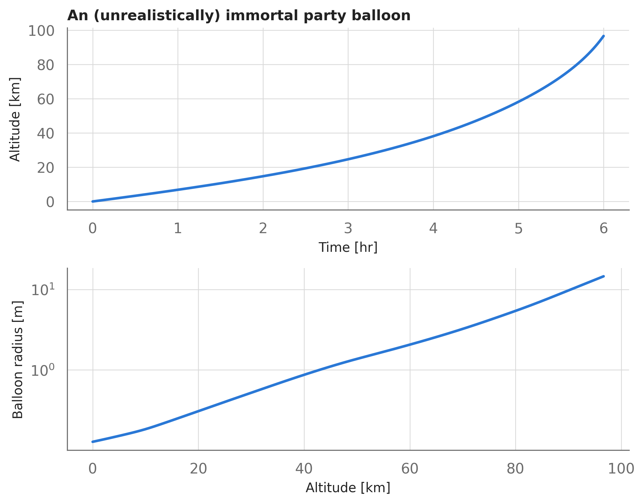
Altitude after 6 hours: 97 km
Balloon radius up there: 14.6 m

Figure 13.9: The balloon ascends at an ever-increasing rate — because in this model it expands without limit as ambient pressure falls, so its buoyant volume grows while drag-per-volume shrinks. The lower panel shows the physically absurd consequence and the real answer: long before reaching these radii, the rubber pops.

The simulation says the balloon rises forever, ever faster — until you look at the radius plot and see why: our infinitely-stretchy balloon has swollen to 14.6 m across. In reality, of course, the rubber bursts within the first couple of kilometers of that curve. It’s a good reminder that an integrator faithfully extrapolates your assumptions, not reality.

One last trick in the same spirit: because a Dynamics instance is just a container of state arrays with aerospace semantics, you can build one from measured data instead of simulation — for instance, loading GPS-logger data from a real flight into a DynamicsPointMass3DSpeedGammaTrack (positions, speed, and track from the log; flight-path and bank angles reconstructed from finite differences) and then calling dyn.draw() for an instant 3D replay of the flight. The dynamics stack doesn’t care where the numbers came from.

13.6 Where to go next

• This chapter leaned on the trajectory-optimization machinery — collocation via constrain_derivative(), free final times, initial guesses as storyboards, and refinement studies — all of which is developed carefully in Section 12.1.
• The Cessna study treated AeroBuildup as a black box that happens to be differentiable. Section 7.3 opens the box: what it models, when to trust it, and the higher-fidelity methods above it.
• Dynamics closes the loop between designing an aircraft and flying it. The complete design studies — especially the transport-aircraft sizing of Section 16.1 — show mission analysis and vehicle design solved simultaneously in a single Opti problem, which is where this stack pays off most.