import aerosandbox as asb
import aerosandbox.numpy as np
import aerosandbox.tools.units as u

opti = asb.Opti()11 Aircraft Sizing: SimPleAC
In this chapter, we size a complete airplane — aerodynamics, wing structure, fuel volume, and mission performance, all coupled — in about 40 lines of model code that solve in milliseconds. Along the way you’ll learn the single most underrated feature of optimization-native design: because the optimizer carries exact derivative information, you get the sensitivity of your objective to every requirement and technology assumption essentially for free, without re-solving anything. We close by cross-checking the optimum against a published geometric-programming (GP) solution of the same problem, and by sweeping the design across a 12× range of missions.
If the previous chapter (Wing Design) was about making a single discipline push back, this chapter is about closure: making a whole vehicle’s weights, aerodynamics, and mission consistent with each other at the optimum.
11.1 The SimPleAC problem
The design brief: a small piston-engine airplane must carry a fixed useful load of 6,250 N (airframe-minus-wing, engine, and payload together) over a 1,000 km mission, and it must be able to take off and land at no more than 25 m/s. Everything else — how big the wing is, how slender it is, how fast to cruise, how much fuel to carry, and where to put that fuel — is up to the optimizer. The objective is to burn as little fuel as possible.
This problem is called SimPleAC (“Simple Aircraft”), proposed by Warren Hoburg and refined in Berk Öztürk’s MIT Master’s thesis. It was created as a showcase for geometric programming via GPKit, and the reference implementation lives in GPLibrary. That pedigree makes it a perfect validation case: a GP solver computes a certified global optimum for this problem, so we can check AeroSandbox’s general-purpose automatic-differentiation (AD) approach against a known answer — and then go beyond what GP can express.
The physics couples in a loop that should feel familiar from any aircraft design text:
- A bigger mission needs more fuel, which adds weight.
- More weight needs more lift, hence more wing area or speed — but the landing-speed requirement pins the wing area to the weight.
- More wing area and span add drag and structural weight, which… burns more fuel.
Sizing means finding the fixed point of this loop, and choosing the free parameters (aspect ratio, cruise speed, fuel placement) to make that fixed point as cheap as possible. In an optimization framework, we don’t iterate the loop manually — we just state all the couplings as constraints and let the optimizer close them simultaneously.
11.2 The model
We begin by creating an optimization environment:
11.2.1 Constants, as parameters
Next, the fixed inputs. We declare each one as an opti.parameter() rather than a plain Python float. For solving, the two are interchangeable — a parameter is just a constant the optimizer never touches. The payoff comes later, in Section 11.5: declaring inputs as parameters lets us extract the sensitivity of the optimum to every one of them after the solve, at negligible cost. All values are in base SI units.
### Environment
g     = opti.parameter(value=9.81)      # gravitational acceleration [m/s^2]
mu    = opti.parameter(value=1.775e-5)  # air viscosity [kg/m/s]
rho   = opti.parameter(value=1.23)      # air density [kg/m^3]
rho_f = opti.parameter(value=817)       # fuel density [kg/m^3]

### Technology assumptions (non-dimensional)
C_Lmax     = opti.parameter(value=1.6)    # max C_L, flaps down [-]
e          = opti.parameter(value=0.92)   # Oswald efficiency factor [-]
k          = opti.parameter(value=1.17)   # form factor [-]
N_ult      = opti.parameter(value=3.3)    # ultimate load factor [-]
S_wetratio = opti.parameter(value=2.075)  # wetted area / reference area [-]
tau        = opti.parameter(value=0.12)   # airfoil thickness-to-chord ratio [-]
W_W_coeff1 = opti.parameter(value=2e-5)   # wing weight coefficient 1 [1/m]
W_W_coeff2 = opti.parameter(value=60)     # wing weight coefficient 2 [Pa]

### Requirements
Range = opti.parameter(value=1000e3)      # mission range [m]
TSFC  = opti.parameter(value=0.6 / u.hour)  # thrust-specific fuel consumption [1/s]
V_min = opti.parameter(value=25)          # takeoff / landing speed limit [m/s]
W_0   = opti.parameter(value=6250)        # fixed weight: everything but wing & fuel [N]
11.2.2 Design variables
Seven quantities are free. Each gets an order-of-magnitude initial guess from engineering intuition (these were chosen before looking at the answer — a cruise-speed guess of 100 m/s turns out to be almost 2× too fast, and it doesn’t matter).
AR       = opti.variable(init_guess=10,    scale=10,    log_transform=True)  # aspect ratio [-]
S        = opti.variable(init_guess=10,    scale=10,    log_transform=True)  # wing area [m^2]
V        = opti.variable(init_guess=100,   scale=100,   log_transform=True)  # cruise speed [m/s]
W        = opti.variable(init_guess=10000, scale=10000, log_transform=True)  # gross weight [N]
C_L      = opti.variable(init_guess=1,     scale=1,     log_transform=True)  # cruise lift coefficient [-]
W_f      = opti.variable(init_guess=3000,  scale=3000,  log_transform=True)  # fuel weight [N]
V_f_fuse = opti.variable(init_guess=1,     scale=1,     log_transform=True)  # fuselage fuel volume [m^3]
Two modeling choices here deserve a comment (both are covered in depth in Building Robust Optimization Models):
log_transform=Truemakes the solver work with \(\ln x\) instead of \(x\). Every one of these quantities is physically positive and appears in power-law-type relations, so log-space is their natural habitat: positivity is enforced automatically, and the singularity at zero (e.g., \(Re \to 0\) in the skin-friction model, or \(AR \to 0\) giving zero span) can never be visited.scale=equal to the initial guess makes the solver-facing log variable exactly \(\ln x\), i.e., unit-scaled — a step of 1 in solver space means an \(e\)-fold change in the physical quantity, for every variable. This costs nothing to write and measurably improves solver robustness, which will matter when we sweep this problem over a wide parameter range in Section 11.6.
Compared to the original GPKit formulation, we also silently dropped several “free variables” (Re, C_f, C_D, D, L/D, T_flight, …) that don’t need to be decision variables at all — they’re explicit functions of the seven above, so we’ll simply compute them. Same engineering problem, simpler notation, smaller problem for the solver.
11.2.3 Weights and lift
The wing’s weight has two parts. The skin weight scales with wing area. The structural (bending) weight grows steeply with aspect ratio — a slender wing is a long lever arm — and with the square root of the product of the loads it must carry: the weight sized by the gust/maneuver load (\(W\), through the ultimate load factor \(N_\mathrm{ult}\)) and the weight providing inertial relief. In symbols:
\[ W_w = \underbrace{W_{W,2} \, S \vphantom{\frac{W}{\tau}}}_{\text{skin}} \;+\; \underbrace{\frac{W_{W,1}}{\tau} \, N_\mathrm{ult} \, A\!R^{3/2} \sqrt{\left(W_0 + \rho_f g V_{f,\mathrm{fuse}}\right) W \, S}}_{\text{bending structure}} \]
Note the appearance of \(\rho_f g V_{f,\mathrm{fuse}}\): fuel stored in the fuselage adds to the load the wing root must carry, whereas fuel stored in the wing provides bending relief. This term is what will make the fuel-placement trade interesting.
Three constraints tie weights to lift:
- Weight closure: gross weight covers fixed weight, wing weight, and fuel.
- Cruise lift: lift equals weight at the mid-cruise point (half the fuel burned).
- Landing: at gross weight, the wing must be able to fly at
V_minwith flaps down — this is what forces the wing to be big.
W_w_surf = W_W_coeff2 * S
W_w_strc = (
    W_W_coeff1 / tau * N_ult * AR**1.5
    * np.sqrt((W_0 + V_f_fuse * rho_f * g) * W * S)
)
W_w = W_w_surf + W_w_strc

opti.subject_to([
    W >= W_0 + W_w + W_f,                                 # weight closure
    W_0 + W_w + 0.5 * W_f <= 0.5 * rho * S * C_L * V**2,  # cruise lift, mid-fuel
    W <= 0.5 * rho * S * C_Lmax * V_min**2,               # stall at landing speed
])
11.2.4 Drag and fuel burn
Drag has three contributions: fuselage form drag (proportional to a drag area \(CDA_0\)), wing profile drag (turbulent flat-plate skin friction with a form factor), and induced drag. A modeling quirk inherited from SimPleAC: the fuselage drag area is tied to the fuselage fuel volume, \(CDA_0 = V_{f,\mathrm{fuse}} / 10\,\mathrm{m}\) — a bigger belly tank means a fatter, draggier fuselage. So fuselage fuel costs drag, and wing fuel costs nothing aerodynamically — but wing volume is limited by the wing’s own geometry. The optimizer will have to balance these.
Fuel burn comes from cruising a distance Range at speed \(V\) with drag \(D\) and a thrust-specific fuel consumption TSFC:
\[ W_f \geq \mathrm{TSFC} \cdot \underbrace{\frac{\mathrm{Range}}{V}}_{\text{flight time}} \cdot \, D \]
This is the Breguet range relation, linearized by evaluating drag at the mid-cruise weight (the 0.5 * W_f in the lift constraint above). For fuel fractions this small the approximation is excellent, and it keeps the model algebraic.
Re  = (rho / mu) * V * np.sqrt(S / AR)  # Reynolds number at mean chord
C_f = 0.074 / Re**0.2                   # turbulent flat-plate skin friction

CDA0 = V_f_fuse / 10                    # fuselage drag area [m^2]

C_D_fuse = CDA0 / S                     # fuselage
C_D_wpar = k * C_f * S_wetratio         # wing profile
C_D_ind  = C_L**2 / (np.pi * AR * e)    # induced
C_D = C_D_fuse + C_D_wpar + C_D_ind

D = 0.5 * rho * V**2 * S * C_D

T_flight = Range / V

opti.subject_to(W_f >= TSFC * T_flight * D)
11.2.5 Fuel volume
The fuel has to physically fit somewhere: in the wing box or in the fuselage tank. The wing’s available volume scales like span × chord × airfoil thickness, i.e., linearly in span and thickness and quadratically in chord, which works out to \(S^{1.5} A\!R^{-0.5} \tau\):
V_f = W_f / (g * rho_f)                        # required tank volume [m^3]
V_f_wing = 0.03 * S**1.5 / np.sqrt(AR) * tau   # volume available in wing box [m^3]

opti.subject_to(V_f_wing + V_f_fuse >= V_f)
11.2.6 Solve
That’s the whole airplane. Minimize fuel and solve:
opti.minimize(W_f)

sol = opti.solve(max_iter=100)
This is Ipopt version 3.14.11, running with linear solver MUMPS 5.4.1.
Number of nonzeros in equality constraint Jacobian...: 0
Number of nonzeros in inequality constraint Jacobian.: 24
Number of nonzeros in Lagrangian Hessian.............: 19
Total number of variables............................: 7
variables with only lower bounds: 0
variables with lower and upper bounds: 0
variables with only upper bounds: 0
Total number of equality constraints.................: 0
Total number of inequality constraints...............: 5
inequality constraints with only lower bounds: 0
inequality constraints with lower and upper bounds: 0
inequality constraints with only upper bounds: 5
iter objective inf_pr inf_du lg(mu) ||d|| lg(rg) alpha_du alpha_pr ls
0 3.0000000e+03 3.85e+03 5.89e+01 0.0 0.00e+00 - 0.00e+00 0.00e+00 0
1 1.6617064e+03 1.68e+03 1.79e+02 -1.2 7.11e-01 2.0 9.92e-01 1.00e+00f 1
2 2.4552629e+03 3.57e+02 3.99e+01 -0.9 8.16e-01 1.5 1.00e+00 8.79e-01h 1
3 2.7647196e+03 4.96e+00 7.08e+00 -0.7 2.52e-01 1.0 1.00e+00 1.00e+00h 1
4 2.7097731e+03 0.00e+00 9.62e+00 -2.6 2.78e-01 0.6 1.00e+00 5.78e-01f 1
5 2.6705232e+03 1.70e-01 1.06e+00 -2.6 8.62e-01 0.1 1.00e+00 9.48e-01f 1
6 2.6077879e+03 9.17e-01 1.08e+00 -3.0 2.63e+00 -0.4 1.00e+00 7.38e-01f 1
7 2.3511820e+03 1.34e+01 1.14e+00 -5.2 8.29e+00 -0.9 1.00e+00 1.00e+00f 1
8 1.4833379e+03 2.10e+02 1.94e+00 -10.2 3.15e+01 -1.3 1.00e+00 9.85e-01f 1
9 1.4627473e+03 2.07e+02 3.29e+01 -3.2 2.02e+01 -0.9 1.00e+00 1.54e-02f 1
iter objective inf_pr inf_du lg(mu) ||d|| lg(rg) alpha_du alpha_pr ls
10 1.4619769e+03 2.07e+02 1.06e+01 -3.2 2.11e+00 - 1.00e+00 1.47e-03h 1
11 1.0909687e+03 9.13e+01 1.91e+00 -5.3 4.18e-01 - 1.00e+00 1.00e+00f 1
12 9.5942303e+02 2.02e+01 7.97e-01 -5.8 2.46e-01 - 1.00e+00 1.00e+00f 1
13 9.3832026e+02 9.58e-01 6.02e-02 -7.4 6.53e-02 - 1.00e+00 1.00e+00h 1
14 9.3775634e+02 1.67e-03 1.27e-04 -9.1 3.28e-03 - 1.00e+00 1.00e+00h 1
15 9.3775596e+02 5.86e-10 2.45e-10 -11.0 6.59e-06 - 1.00e+00 1.00e+00h 1
Number of Iterations....: 15
(scaled) (unscaled)
Objective...............: 3.1258531841321052e+01 9.3775595523963079e+02
Dual infeasibility......: 2.4453328251183848e-10 7.3359984753551486e-09
Constraint violation....: 8.2564139401092708e-12 5.8560883393511031e-10
Variable bound violation: 0.0000000000000000e+00 0.0000000000000000e+00
Complementarity.........: 1.0000306005617723e-11 3.0000918016853143e-10
Overall NLP error.......: 2.4453328251183848e-10 7.3359984753551486e-09
Number of objective function evaluations = 16
Number of objective gradient evaluations = 16
Number of equality constraint evaluations = 0
Number of inequality constraint evaluations = 16
Number of equality constraint Jacobian evaluations = 0
Number of inequality constraint Jacobian evaluations = 16
Number of Lagrangian Hessian evaluations = 15
Total seconds in IPOPT = 0.041
EXIT: Optimal Solution Found.
solver : t_proc (avg) t_wall (avg) n_eval
nlp_f | 1.24ms ( 77.31us) 139.53us ( 8.72us) 16
nlp_g | 8.03ms (501.81us) 757.16us ( 47.32us) 16
nlp_grad_f | 2.09ms (123.00us) 235.89us ( 13.88us) 17
nlp_hess_l | 14.38ms (959.00us) 1.67ms (111.66us) 15
nlp_jac_g | 10.45ms (615.00us) 1.12ms ( 65.76us) 17
total | 413.18ms (413.18ms) 42.65ms ( 42.65ms) 1IPOPT closes the entire coupled sizing loop in 15 iterations — note the Total seconds in IPOPT line above: the solve itself takes a few tens of milliseconds. (The first call to opti.solve() also spends a moment building and compiling the computational graph; re-solves at new parameter values skip that and run at nearly the raw IPOPT speed, which we’ll exploit shortly.)
11.3 The optimal airplane
Let’s see what the optimizer designed:
b = np.sqrt(AR * S)  # wingspan [m]

print("Design variables:")
for name, x, unit in [
    ("Aspect ratio",         AR,       "-"),
    ("Wing area",            S,        "m^2"),
    ("Cruise speed",         V,        "m/s"),
    ("Gross weight",         W,        "N"),
    ("Cruise C_L",           C_L,      "-"),
    ("Fuel weight",          W_f,      "N"),
    ("Fuselage fuel volume", V_f_fuse, "m^3"),
]:
    print(f"    {name:22s} = {sol(x):10.4g} {unit}")

print("Derived quantities:")
for name, x, unit in [
    ("Wingspan",             b,               "m"),
    ("Gross mass",           W / g,           "kg"),
    ("Fuel fraction",        W_f / W,         "-"),
    ("Wing weight",          W_w,             "N"),
    ("  ...structural part", W_w_strc,        "N"),
    ("Cruise L/D",           C_L / C_D,       "-"),
    ("Cruise Reynolds no.",  Re,              "-"),
    ("Drag",                 D,               "N"),
    ("Flight time",          T_flight / u.hour, "hr"),
    ("Wing fuel volume",     V_f_wing,        "m^3"),
    ("Total fuel volume",    V_f,             "m^3"),
]:
    print(f"    {name:22s} = {sol(x):10.4g} {unit}")
Design variables:
Aspect ratio = 12.1 -
Wing area = 14.15 m^2
Cruise speed = 57.11 m/s
Gross weight = 8705 N
Cruise C_L = 0.2901 -
Fuel weight = 937.8 N
Fuselage fuel volume = 0.0619 m^3
Derived quantities:
Wingspan = 13.09 m
Gross mass = 887.3 kg
Fuel fraction = 0.1077 -
Wing weight = 1517 N
...structural part = 667.8 N
Cruise L/D = 25.63 -
Cruise Reynolds no. = 4.279e+06 -
Drag = 321.3 N
Flight time = 4.864 hr
Wing fuel volume = 0.0551 m^3
Total fuel volume = 0.117 m^3This is a thoroughly sensible airplane: a 887 kg, 13.1 m-span machine — Cessna-172 class — cruising at 57 m/s. Several features of the optimum are worth reading closely:
- The wing is sized by the landing requirement. At 8705 N of lift at 25 m/s with \(C_{L,\max}\) flaps, the stall constraint is exactly active. Cruise then happens at a low \(C_L\) of 0.29 — the wing is “too big” for cruise because the runway, not the cruise, set its size.
- The fuel splits between wing and fuselage. Of the 117 L of fuel, 55 L rides in the wing (free bending relief, no drag) and 62 L in the fuselage. The optimizer stops adding fuselage volume exactly where the marginal drag cost of a fatter fuselage balances the marginal structural cost of carrying fuel in the wing… a trade you would not want to close by hand.
- The airplane does not fly at its best L/D. Cruise L/D is 25.6, noticeably below the airframe’s maximum. That is not a mistake, and the next figure shows why.
Code
import _common
import matplotlib.pyplot as plt

# Freeze the optimized design (geometry, weights), then trim it across speeds:
V_grid = np.linspace(35, 90, 500)                    # candidate cruise speeds [m/s]
q = 0.5 * sol(rho) * V_grid**2                       # dynamic pressure [Pa]
CL_trim = sol(W_0 + W_w + 0.5 * W_f) / (q * sol(S))  # C_L required for L = W
Re_grid = sol(rho / mu) * V_grid * np.sqrt(sol(S / AR))

D_fuse = q * sol(CDA0)
D_prof = q * sol(S) * sol(k * S_wetratio) * 0.074 / Re_grid**0.2
D_ind  = q * sol(S) * CL_trim**2 / (np.pi * sol(AR * e))
D_trim = D_fuse + D_prof + D_ind

fuel_per_km = sol(TSFC) * D_trim / V_grid * 1e3      # fuel weight per distance [N/km]

V_star = sol(V)
V_minD = V_grid[np.argmin(D_trim)]

fig, (ax1, ax2) = plt.subplots(2, 1, figsize=(7, 6.8), sharex=True)

c = _common.SERIES
ax1.plot(V_grid, D_trim, color=c[0])
ax1.plot(V_grid, D_ind, color=_common.TEXT_SECONDARY, lw=1.2)
ax1.plot(V_grid, D_prof, color=_common.TEXT_SECONDARY, lw=1.2)
ax1.plot(V_grid, D_fuse, color=_common.TEXT_SECONDARY, lw=1.2)
_common.label_line(ax1, V_grid[-1], D_trim[-1], "total", c[0], dx=1)
_common.label_line(ax1, V_grid[0], D_ind[0], "induced", _common.TEXT_SECONDARY,
                   dx=1, dy=25)
_common.label_line(ax1, V_grid[-1], D_prof[-1], "wing profile", _common.TEXT_SECONDARY, dx=1)
_common.label_line(ax1, V_grid[-1], D_fuse[-1], "fuselage", _common.TEXT_SECONDARY, dx=1)
ax1.set_ylabel("Drag [N]")
ax1.set_title("Minimum drag is at low speed...")
ax1.set_ylim(bottom=0)

ax2.plot(V_grid, fuel_per_km, color=c[0])
ax2.set_xlabel("Cruise speed [m/s]")
ax2.set_ylabel("Fuel burned per distance [N/km]")
ax2.set_title("...but minimum fuel-per-distance is what the mission rewards")
ax2.set_ylim(bottom=0)

for ax in (ax1, ax2):
    ax.axvline(V_minD, color=_common.TEXT_SECONDARY, lw=0.8, ls="--", zorder=0)
    ax.axvline(V_star, color=c[3], lw=0.8, ls="--", zorder=0)
ax1.text(V_minD, ax1.get_ylim()[1] * 0.97, " min drag\n (best glide)",
         color=_common.TEXT_SECONDARY, va="top", fontsize=8)
ax1.text(V_star, ax1.get_ylim()[1] * 0.97, " chosen cruise",
         color=c[3], va="top", fontsize=8)

plt.subplots_adjust(right=0.85, hspace=0.35)
plt.show()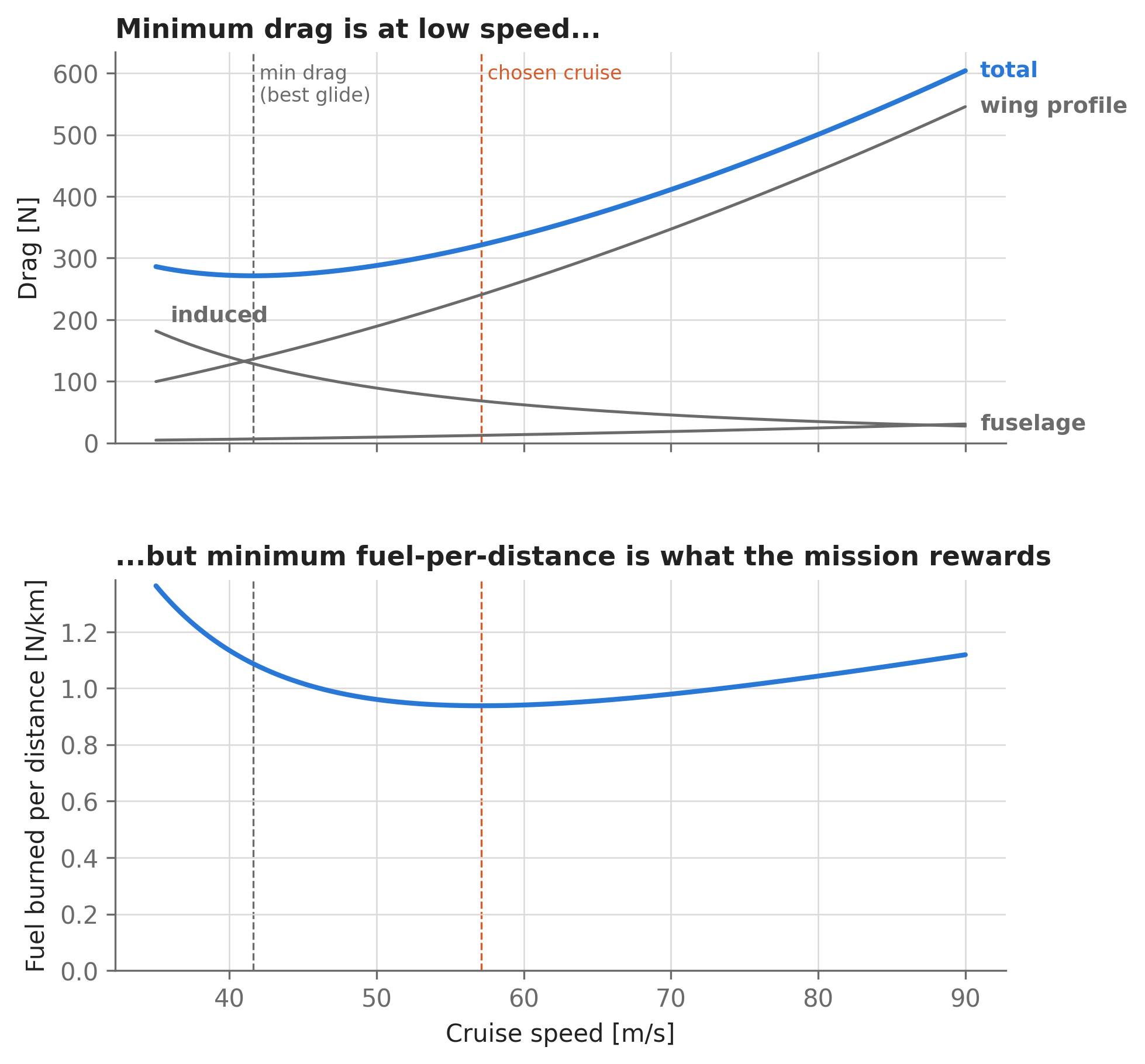
Because total fuel equals (fuel per distance) × (range), the optimizer minimizes \(D/V\), not \(D\) — and the \(D/V\) minimum sits at 57.2 m/s, essentially exactly the chosen cruise speed of 57.1 m/s. Induced drag falls with speed while profile drag rises; dividing by \(V\) shifts the balance point toward higher speed. This is the classic result that best-range speed is faster than best-endurance/best-glide speed, discovered here by a nonlinear program rather than told to it.
11.4 Cross-check: geometric programming agrees
SimPleAC’s authors solved this problem with GPKit, which transforms it into a (log-space convex) geometric program and returns a certified globally optimal solution. That printed solution gives us a rare thing in design optimization: ground truth to compare against.
from IPython.display import Markdown

# GPKit's solution, transcribed from the original SimPleAC run
# (github.com/convexengineering/gplibrary, SP/SimPleAC; printed to 3-4 sig. figs):
comparison = [
    # quantity            unit    AeroSandbox value       GPKit value
    ("Aspect ratio",      "-",    sol(AR),                12.1),
    ("Wing area",         "m^2",  sol(S),                 14.15),
    ("Cruise speed",      "m/s",  sol(V),                 57.11),
    ("Gross weight",      "N",    sol(W),                 8705),
    ("Cruise C_L",        "-",    sol(C_L),               0.2901),
    ("Fuel weight",       "N",    sol(W_f),               937.8),
    ("Fuselage tank",     "m^3",  sol(V_f_fuse),          0.0619),
    ("Wing tank",         "m^3",  sol(V_f_wing),          0.0551),
    ("Drag",              "N",    sol(D),                 321.3),
    ("Drag coefficient",  "-",    sol(C_D),               0.01132),
    ("Skin friction",     "-",    sol(C_f),               0.003491),
    ("Fuselage drag area","m^2",  sol(CDA0),              0.00619),
    ("Cruise L/D",        "-",    sol(C_L / C_D),         25.63),
    ("Reynolds number",   "-",    sol(Re),                4.279e6),
    ("Flight time",       "hr",   sol(T_flight) / u.hour, 4.864),
    ("Fuel volume",       "m^3",  sol(V_f),               0.117),
    ("Wing weight",       "N",    sol(W_w),               1517),
    ("... structural",    "N",    sol(W_w_strc),          667.8),
    ("... skin",          "N",    sol(W_w_surf),          849.2),
]

Markdown(
    "| Quantity | Unit | AeroSandbox | GPKit | Rel. difference |\n"
    "|:---|:---|---:|---:|---:|\n"
    + "\n".join(
        f"| {name} | {unit} | {asb_val:.6g} | {gp_val:.4g} | {asb_val / gp_val - 1:+.2e} |"
        for name, unit, asb_val, gp_val in comparison
    )
)| Quantity | Unit | AeroSandbox | GPKit | Rel. difference |
|---|---|---|---|---|
| Aspect ratio | - | 12.1049 | 12.1 | +4.04e-04 |
| Wing area | m^2 | 14.1542 | 14.15 | +2.95e-04 |
| Cruise speed | m/s | 57.106 | 57.11 | -6.96e-05 |
| Gross weight | N | 8704.82 | 8705 | -2.10e-05 |
| Cruise C_L | - | 0.290128 | 0.2901 | +9.65e-05 |
| Fuel weight | N | 937.756 | 937.8 | -4.70e-05 |
| Fuselage tank | m^3 | 0.0619038 | 0.0619 | +6.13e-05 |
| Wing tank | m^3 | 0.0550997 | 0.0551 | -5.93e-06 |
| Drag | N | 321.309 | 321.3 | +2.82e-05 |
| Drag coefficient | - | 0.0113188 | 0.01132 | -1.08e-04 |
| Skin friction | - | 0.00349109 | 0.003491 | +2.70e-05 |
| Fuselage drag area | m^2 | 0.00619038 | 0.00619 | +6.13e-05 |
| Cruise L/D | - | 25.6325 | 25.63 | +9.57e-05 |
| Reynolds number | - | 4.27908e+06 | 4.279e+06 | +1.92e-05 |
| Flight time | hr | 4.86425 | 4.864 | +5.07e-05 |
| Fuel volume | m^3 | 0.117003 | 0.117 | +2.97e-05 |
| Wing weight | N | 1517.06 | 1517 | +4.05e-05 |
| … structural | N | 667.811 | 667.8 | +1.64e-05 |
| … skin | N | 849.25 | 849.2 | +5.94e-05 |
Every quantity matches to within GPKit’s printed precision — the largest relative difference across all 19 quantities is 4.0e-04, which is rounding in GPKit’s 3-to-4-significant-figure output, not real disagreement. Both solvers drive their own convergence tolerances far tighter than this. Since the GP solution is provably the global optimum of this problem, we’ve confirmed that the AD/IPOPT approach landed on the global optimum here too.
It’s worth being precise about what each approach buys you, since “GP vs. NLP” is a recurring design decision in this field:
- Speed: comparable, and both are effectively instant at this scale (milliseconds). The AD approach also solved a smaller problem here, since intermediate quantities didn’t need to be decision variables.
- Guarantees: GP certifies global optimality — of a GP-compatible model. If your true physics isn’t GP-compatible (transonic drag rise, stall, tabulated engine decks, …), you must either approximate it with GP-compatible surrogates — at which point the certificate applies to the approximation, not your problem — or abandon the guarantee via signomial programming. The AD approach never had the certificate, but it also never restricted what you’re allowed to write: any differentiable model, including everything in the rest of this book, is fair game.
- Robustness: GP needs no initial guess; the AD approach converges reliably given order-of-magnitude guesses (ours were off by up to 2× and it did not matter), but can fail if guesses are wildly wrong. Engineering intuition is usually more than sufficient.
In short: when a problem is GP-compatible, both methods find the same answer at the same speed; when it isn’t, only one of them can express it. For a fuller treatment of solver behavior and failure modes, see Solvers and Solutions.
11.5 Sensitivities for free
Here’s the question every design review actually asks: “What’s that requirement costing us?” If the landing-speed requirement were relaxed by 5%, how much fuel would we save? What if the engine’s TSFC improved by 10%? Is empty weight or drag the better place to spend engineering effort?
The remarkable fact is that the optimizer has already computed all of these answers. At a constrained optimum, each constraint carries a Lagrange multiplier (a dual variable or shadow price): the rate at which the optimal objective would improve if that constraint were relaxed. IPOPT computes these as part of solving the problem. Formally, if the problem is
\[ J^*(p) = \min_x \; f(x, p) \quad \text{s.t.} \quad g(x, p) \leq 0, \]
with parameters \(p\), then the envelope theorem (equivalently, first-order NLP sensitivity analysis) says
\[ \frac{\mathrm{d}J^*}{\mathrm{d}p} = \frac{\partial f}{\partial p} + \lambda^\top \frac{\partial g}{\partial p} = \frac{\partial \mathcal{L}}{\partial p}, \]
evaluated at the optimum — the total derivative of the optimal cost, accounting for how the entire optimal design re-arranges itself, equals a partial derivative of the Lagrangian \(\mathcal{L} = f + \lambda^\top g\), which needs no re-solving at all. This is why we declared the constants as opti.parameter()s: AeroSandbox’s Opti is a thin subclass of CasADi’s, so we can drop one level down and evaluate this expression symbolically.
One more transformation makes the result maximally readable. Raw derivatives have awkward units (\(\mathrm{d}W_f / \mathrm{d}\,\mathrm{TSFC}\) is in newton-seconds…). Instead we report log-log sensitivities,
\[ \hat{S}_p \;=\; \frac{\mathrm{d}\ln J^*}{\mathrm{d}\ln p} \;=\; \frac{p}{J^*}\frac{\mathrm{d}J^*}{\mathrm{d}p}, \]
read as “a 1% increase in \(p\) produces an \(\hat{S}_p\)% increase in optimal fuel burn” — dimensionless, comparable across parameters, and exactly the sensitivity format GPKit reports.
import casadi as cas

constants = {
    "g": g, "mu": mu, "rho": rho, "rho_f": rho_f,
    "C_Lmax": C_Lmax, "e": e, "k": k, "N_ult": N_ult,
    "S_wetratio": S_wetratio, "tau": tau,
    "W_W_coeff1": W_W_coeff1, "W_W_coeff2": W_W_coeff2,
    "Range": Range, "TSFC": TSFC, "V_min": V_min, "W_0": W_0,
}

lagrangian = opti.f + cas.dot(opti.lam_g, opti.g)

sens = {  # d(ln J*) / d(ln p) for each parameter p
    name: float(sol(cas.gradient(lagrangian, p) * p / opti.f))
    for name, p in constants.items()
}

for name, s in sorted(sens.items(), key=lambda item: -abs(item[1])):
    print(f"{name:12s} {s:+7.3f}")
V_min -1.311
Range +1.199
TSFC +1.199
W_0 +0.936
S_wetratio +0.898
k +0.898
C_Lmax -0.655
e -0.255
mu +0.180
rho -0.146
tau -0.140
W_W_coeff2 +0.121
N_ult +0.095
W_W_coeff1 +0.095
rho_f -0.091
g -0.091Code
import _common
import matplotlib.pyplot as plt

names, vals = zip(*sorted(sens.items(), key=lambda item: abs(item[1])))
colors = [_common.SERIES[3] if v > 0 else _common.SERIES[0] for v in vals]

fig, ax = plt.subplots(figsize=(7, 5.2))
ax.barh(names, vals, color=colors, height=0.65)
for i, v in enumerate(vals):
    ax.text(v + (0.03 if v > 0 else -0.03), i, f"{v:+.2f}",
            va="center", ha="left" if v > 0 else "right",
            fontsize=8, color=_common.TEXT_PRIMARY)
ax.set_xlabel("Fuel-burn sensitivity  d ln($W_f$) / d ln($p$)  [-]")
ax.set_title("Where the fuel burn comes from")
ax.set_xlim(-1.75, 1.75)
ax.axvline(0, color=_common.TEXT_SECONDARY, lw=0.8)
ax.text(1.7, len(vals) - 0.5, "more fuel →", color=_common.SERIES[3],
        ha="right", fontsize=8, fontweight="bold")
ax.text(-1.7, len(vals) - 0.5, "← less fuel", color=_common.SERIES[0],
        ha="left", fontsize=8, fontweight="bold")
plt.show()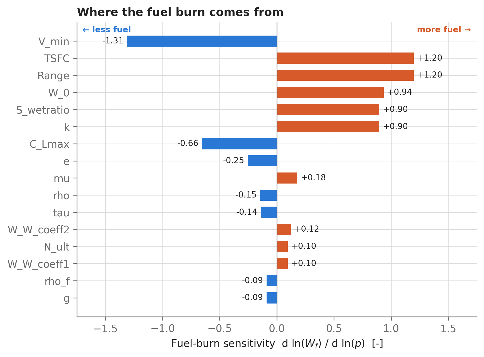
This chart repays close reading — it is, in effect, an audit of the whole design problem:
- The landing-speed requirement is the most expensive line in the spec. \(\hat{S}_{V_\min} =\) -1.31: every 1% of allowed landing speed buys 1.31% of fuel, because it shrinks the wing that the runway — not the cruise — is sizing. If a design review is looking for requirements to challenge, the duals point straight at this one. Relatedly, better flaps (\(C_{L,\max}\), -0.66) buy fuel for exactly the same reason.
- Range and TSFC compound beyond 1:1. Both sit at +1.20: a 1% longer mission costs 1.20% more fuel, because extra fuel adds weight, which adds structure and drag, which adds fuel — the Breguet spiral, priced exactly.
- Empty weight passes through at almost exactly 1:1 (\(\hat{S}_{W_0} =\) +0.94), and profile drag (\(k\), \(S_\mathrm{wet}/S\)) at +0.90 — a useful exchange rate between the structures group and the aero group.
- Parameters that only ever appear multiplied together have identical sensitivities — compare
Range&TSFC,k&S_wetratio,N_ult&W_W_coeff1,g&rho_f. The duals are rediscovering the model’s nondimensional structure: only the products matter, so their log-sensitivities must match. - Sensitivities audit your assumptions. Gravity has a negative sensitivity (-0.09) — stronger gravity means less fuel?! It’s correct, given what the model holds fixed: \(W_0\) is specified as a weight, so heavier gravity doesn’t make the airplane heavier; the only surviving effect is that the same fuel weight occupies less volume (\(V_f = W_f / \rho_f g\)), shrinking the draggy fuselage tank. A surprising sign in a sensitivity table is usually the model telling you precisely which assumption you forgot you made.
As a check that these dual-based numbers mean what we claim, compare against a brute-force finite difference — re-solve the whole problem with the range requirement stretched 2% and measure the fuel change:
R_0 = sol(Range)

sol_perturbed = opti.solve(
    parameter_mapping={Range: 1.02 * R_0},  # re-solve at 102% range
    verbose=False,
)

sens_fd = np.log(sol_perturbed(W_f) / sol(W_f)) / np.log(1.02)

print(f"d(ln W_f)/d(ln Range),  from duals            : {sens['Range']:.4f}")
print(f"d(ln W_f)/d(ln Range),  finite difference (+2%): {sens_fd:.4f}")
d(ln W_f)/d(ln Range), from duals : 1.1989
d(ln W_f)/d(ln Range), finite difference (+2%): 1.2012They agree to 0.2% (the small residual is real curvature across the 2% step, not error). The difference in cost is the point: the finite difference needed a full re-solve per parameter, per direction; the duals priced all 16 parameters simultaneously, using only information the original solve already had.
11.6 From local sensitivities to design sweeps
Duals give the slope of the optimal-cost curve at one point. To see the whole curve — “what does the 2,500 km version of this airplane look like?” — we re-solve across a parameter range. Because each re-solve starts from a compiled problem, this is cheap; the craft is in making it reliable. Two practices help (both discussed further in Solvers and Solutions):
- Sweep by continuation: walk outward from the solved nominal point, warm-starting each solve from its neighbor’s solution via
opti.set_initial_from_sol(), so the solver always starts near an optimum. - Warm-start the primal variables only (
initialize_duals=False): re-using converged duals from a different parameter value tends to hurt interior-point methods more than it helps.
ranges = np.linspace(250e3, 3000e3, 30)  # mission ranges to study [m]

sweep = {}
for direction in [+1, -1]:  # walk up from the nominal range, then down
    last_sol = sol
    to_solve = ranges[ranges > R_0] if direction > 0 else ranges[ranges <= R_0][::-1]
    for R in to_solve:
        opti.set_initial_from_sol(last_sol, initialize_duals=False)
        last_sol = opti.solve(parameter_mapping={Range: R}, verbose=False)
        sweep[R] = last_sol

print(f"Re-designed the airplane for {len(sweep)} different missions.")
Re-designed the airplane for 30 different missions.All 30 solves converge — a 12× spread in mission range, each point a fully re-optimized airplane. (For one-liner sweeps, opti.solve_sweep() packages this pattern; the explicit loop shown here gives you control over ordering and warm starts when a problem needs coaxing.)
Code
import _common
import matplotlib.pyplot as plt

Rs = np.array(sorted(sweep.keys()))
get = lambda x: np.array([sweep[R](x) for R in Rs])
Wf_sweep = get(W_f)

Rs_km = Rs / 1e3
R_0_km = R_0 / 1e3
Wf_pred = sol(W_f) * (Rs / R_0) ** sens["Range"]  # dual-implied power law

c = _common.SERIES
fig, (ax1, ax2) = plt.subplots(2, 1, figsize=(7, 6.8), sharex=True)

ax1.plot(Rs_km, Wf_sweep, color=c[0])
ax1.plot(Rs_km, Wf_pred, color=c[2], ls="--", lw=1.5)
ax1.plot(R_0_km, sol(W_f), "o", color=c[3], ms=6, zorder=5)
ax1.annotate("nominal design\n(1,000 km)", xy=(R_0_km, sol(W_f)),
             xytext=(R_0_km + 60, sol(W_f) + 900), color=c[3], fontsize=8)
_common.label_line(ax1, Rs_km[-1], Wf_sweep[-1], "re-optimized\nat each range", c[0], dx=25)
_common.label_line(
    ax1, Rs_km[-1], Wf_pred[-1],
    f"dual extrapolation:\n$W_f \\propto R^{{{sens['Range']:.2f}}}$", c[2], dx=25,
)
ax1.set_ylabel("Fuel weight [N]")
ax1.set_title("The dual predicts the trend; re-solving gives the truth")
ax1.set_ylim(bottom=0)

for y, color, ls, name, dy in [
    (get(W) / sol(W), c[4], "-", "gross weight", -0.04),
    (get(S) / sol(S), c[1], "--", "wing area", +0.03),
    (get(AR) / sol(AR), _common.TEXT_SECONDARY, "-", "aspect ratio", 0),
    (get(V) / sol(V), c[3], "-", "cruise speed", 0),
]:
    ax2.plot(Rs_km, y, color=color, ls=ls)
    _common.label_line(ax2, Rs_km[-1], y[-1], name, color, dx=25, dy=dy)
ax2.axhline(1, color=_common.GRID, lw=0.8)

# Mark where the fuel-volume constraint becomes active:
vol_slack = get(V_f_wing + V_f_fuse - V_f)
kink_R_km = Rs_km[np.argmax(vol_slack < 1e-6)]
ax2.axvline(kink_R_km, color=_common.TEXT_SECONDARY, lw=0.8, ls=":", zorder=0)
ax2.text(kink_R_km + 30, 1.42, "fuselage tank\nneeded →",
         color=_common.TEXT_SECONDARY, fontsize=8)

ax2.set_xlabel("Mission range [km]")
ax2.set_ylabel("Relative to nominal design [-]")
ax2.set_title("Every point is a different airplane")

plt.subplots_adjust(right=0.82, hspace=0.3)
plt.show()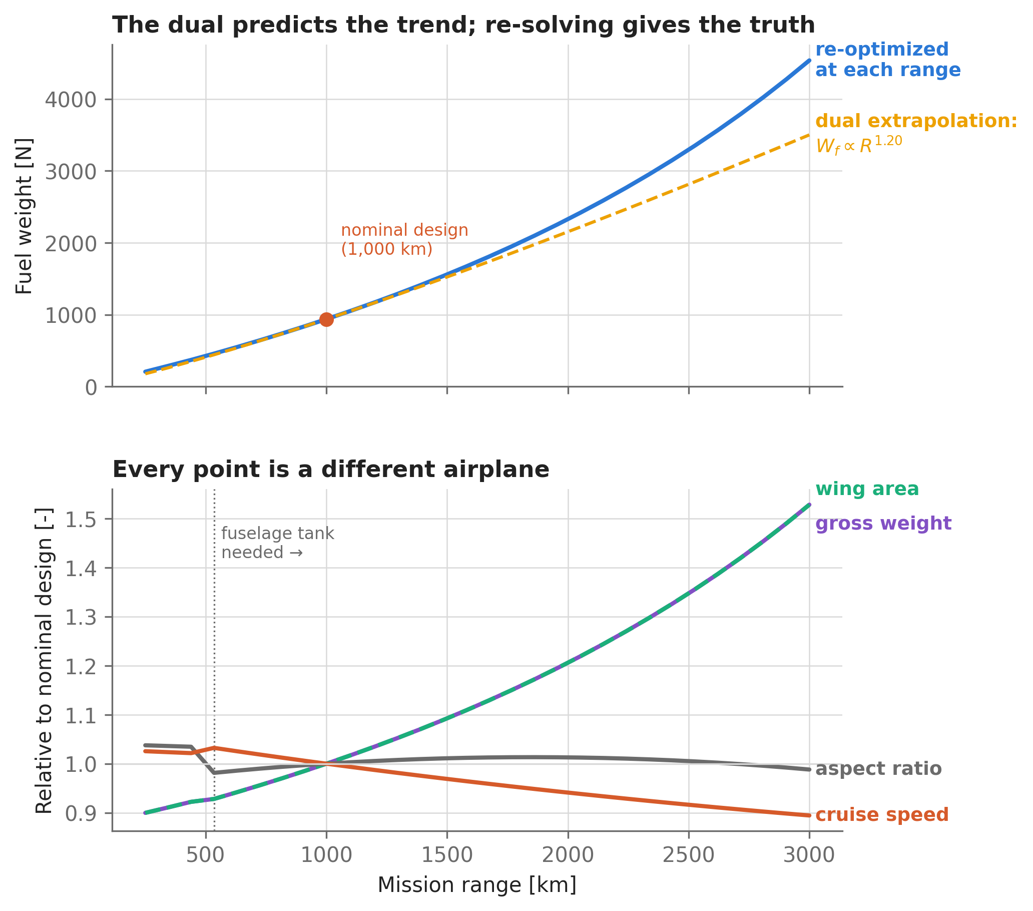
local_exponent = np.log(Wf_sweep[-1] / Wf_sweep[-2]) / np.log(Rs[-1] / Rs[-2])
extrap_error = Wf_pred[-1] / Wf_sweep[-1] - 1
The two views are complementary. Near the nominal point, the dual-implied power law — \(W_f \propto R^{\hat{S}}\) with \(\hat{S} =\) 1.20 — tracks the true re-optimized curve closely — the dual really is the local exponent of the design’s cost growth. Far from it, the extrapolation drifts: by 3,000 km it underpredicts fuel burn by 23%, because the exponent itself grows along the sweep (the local slope between the last two sweep points is already 1.85) as the Breguet weight spiral compounds. Meanwhile, the bottom panel shows the design responding: the 3,000 km airplane carries 4.8× the fuel of the nominal one with 1.5× the wing area, and cruises about 11% slower — while the optimal aspect ratio barely moves. Duals for local exchange rates, sweeps for global trades: use both.
The bottom panel also holds two structural lessons about reading sweeps of optima:
- The wing-area curve (dashed) lies exactly on top of the gross-weight curve. That’s not coincidence: the landing constraint stays binding at every single range, pinning the wing loading of all 30 airplanes at \(W/S = \tfrac{1}{2}\rho \, C_{L,\max} V_\min^2 =\) 615 Pa. The runway sizes the wing for the 250 km airplane exactly as it does for the 3,000 km one, so wing area simply is gross weight in disguise.
- The kink near 534 km marks a constraint-activity change. Below it, the mission’s fuel fits entirely inside the wing box: the optimizer shrinks the fuselage tank — and with it, this model’s fuselage drag — essentially to zero. Above it, fuel spills into the fuselage, and every additional kilometer of range now buys drag as well as weight. Sweeps of optimal designs are typically piecewise-smooth, and each kink flags a qualitative change in what is limiting the design — they’re worth hunting down and explaining, every time.
11.7 Where to go next
This chapter completes the core design-optimization pattern of this book: write physics as constraints, let the optimizer close the loops, then interrogate the optimum (duals, sweeps) rather than just admiring it. From here:
- Solvers and Solutions goes deeper on the machinery used here — parameters and duals, warm starts, sweep tooling, and what to do when a solve fails.
- The complete design studies scale this same pattern up: an aerostructural wing where the “wing weight model” becomes an actual coupled beam + VLM analysis, and a transport aircraft where the weight buildup grows to ~25 components with real engine and aero models.
- If the wing-weight or drag models here felt too coarse, Structures and Aircraft Aerodynamics show the higher-fidelity, still-differentiable models that can drop into exactly this formulation.