16  Sizing a Solar-Electric HALE UAV

This chapter builds a complete sizing tool for a solar-electric high-altitude long-endurance (HALE) aircraft — an “atmospheric satellite” that stays aloft indefinitely by harvesting sunlight — in roughly a hundred lines of model code. Along the way, you’ll see how to couple solar energy collection, battery storage, aerodynamics, propulsion, and structural weight through a single asb.Opti instance, and how to use AeroSandbox’s built-in solar, wind, and mass-model libraries. The formulation here is written fresh for this book, in the spirit of the MIT Dawn aircraft — a flight-proven solar HALE design whose AeroSandbox-based conceptual sizing is documented publicly in the open-source Dawn Design Tool — but deliberately simplified to a single design point so that the whole thing fits on a page and solves in seconds.

16.1 The mission: an airplane that never lands

A solar HALE aircraft loiters in the stratosphere for weeks or months, carrying a small payload — a climate-science instrument, a communications relay, a wildfire-monitoring camera. The requirements we’ll design to are modeled on the publicly-documented Dawn mission:

• Payload: 30 kg science package, drawing 250 W continuously.
• Altitude: at or above 18,288 m (60,000 ft) — above weather, clouds, and nearly all air traffic.
• Station-keeping: able to hold position over a target at 35° N latitude, which requires airspeed to exceed the local 95th-percentile wind speed.
• Endurance: indefinite. The aircraft must end every 24-hour cycle with at least as much stored energy as it started with.

That last requirement — diurnal energy closure — is the crux of the whole problem. During the day, the wing’s solar cells collect more power than the aircraft consumes; the surplus charges a battery. At night, the battery alone must carry the aircraft through until sunrise. If the design can bank enough energy by sunset to survive the night, it can (in principle) fly forever. If it can’t, no amount of piloting skill will save it.

One requirement will look odd: we will minimize wingspan, not weight or cost. This choice comes straight from the Dawn program’s experience: historically, the dominant failure mode of large solar aircraft has been aeroelastic (Helios, Solara 50, Aquila, and Zephyr all suffered in-flight structural or aeroelastic failures), and span is a good first-order proxy for that risk — as well as for very practical headaches like runway width, ground handling, and transport.

16.2 The physics: cheap to collect, expensive to store

Before writing the optimization problem, let’s build intuition for the energy balance using AeroSandbox’s solar library (aerosandbox.library.power_solar). Its main entry point is solar_flux(), which computes the solar power per unit area falling on a (possibly tilted) panel as a function of latitude, day of year, time after solar noon, and altitude — accounting for Earth’s orbital eccentricity, axial tilt, atmospheric absorption and scattering along the slant path, and diffuse re-scattered illumination.

import aerosandbox as asb
import aerosandbox.numpy as np
import aerosandbox.tools.units as u
from aerosandbox.library import power_solar as solar

latitude = 35     # [deg] station-keeping latitude
day_of_year = 172 # June 21, the summer solstice

# Sanity checks against well-known values:
flux_toa = solar.solar_flux_outside_atmosphere_normal(day_of_year)
flux_noon_sea_level = solar.solar_flux(latitude, day_of_year, time=0)
flux_noon_stratosphere = solar.solar_flux(latitude, day_of_year, time=0, altitude=20e3)
night_hours = 24 - solar.length_day(latitude, day_of_year) / u.hour

print(f"Top-of-atmosphere normal flux on this day:   {flux_toa:4.0f} W/m^2")
print(f"Noon flux on a horizontal panel, sea level:  {flux_noon_sea_level:4.0f} W/m^2")
print(f"Noon flux on a horizontal panel, 20 km MSL:  {flux_noon_stratosphere:4.0f} W/m^2")
print(f"Night duration at 35 deg N on the solstice:  {night_hours:.1f} hours")

Top-of-atmosphere normal flux on this day:   1321 W/m^2
Noon flux on a horizontal panel, sea level:  1001 W/m^2
Noon flux on a horizontal panel, 20 km MSL:  1253 W/m^2
Night duration at 35 deg N on the solstice:  9.6 hours

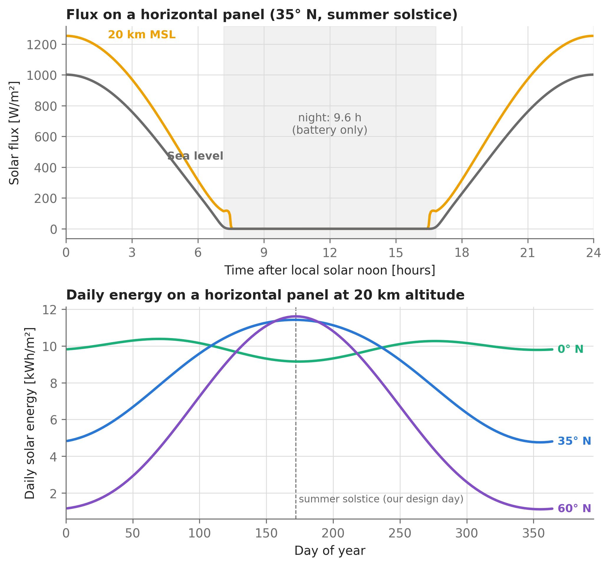
These numbers behave as documented: at sea level the model reproduces the familiar ~1 kW/m² “peak sun”, and at 20 km — above 95% of the atmosphere’s mass — the panel recovers 95% of the top-of-atmosphere flux (the small remaining deficit is the slight off-normal sun angle at 35° N plus residual atmospheric absorption). Figure 16.1 shows the full picture: the daily flux profile at altitude, and how the daily integrated energy varies across the year. The seasonal cliff in the second panel is the single most important feature of the solar-aircraft design space: a mission that closes comfortably in June may be hopeless in December.

import _common
import matplotlib.pyplot as plt

fig, ax = plt.subplots(2, 1, figsize=(7, 6.5))

### Top panel: flux vs. time of day, at two altitudes
t = np.linspace(0, 86400, 500)
hours = t / u.hour
for alt, color, name, x_lab, dy_lab in [
    (20e3, _common.SERIES[2], "20 km MSL", 1.5, 80),
    (0, _common.TEXT_SECONDARY, "Sea level", 4.2, -90),
]:
    flux = solar.solar_flux(latitude, day_of_year, time=t, altitude=alt)
    ax[0].plot(hours, flux, color=color)
    _common.label_line(ax[0], x=x_lab, y=solar.solar_flux(latitude, day_of_year,
                       time=x_lab * u.hour, altitude=alt), text=name, color=color,
                       dx=0.4, dy=dy_lab)
sunset = solar.length_day(latitude, day_of_year) / 2 / u.hour
ax[0].axvspan(sunset, 24 - sunset, color=_common.GRID, alpha=0.35, zorder=0)
ax[0].text(12, 620, f"night: {night_hours:.1f} h\n(battery only)",
           ha="center", color=_common.TEXT_SECONDARY, fontsize=9)
ax[0].set_xlim(0, 24)
ax[0].set_xticks(np.arange(0, 25, 3))
ax[0].set_xlabel("Time after local solar noon [hours]")
ax[0].set_ylabel("Solar flux [W/m²]")
ax[0].set_title("Flux on a horizontal panel (35° N, summer solstice)")

### Bottom panel: daily integrated energy vs. day of year, at three latitudes
days = np.arange(1, 366, 3)
t_col = t[:, None]  # broadcast: (time, day) grid
dt = np.diff(t)[:, None]
for lat_i, color in [(0, _common.SERIES[1]), (35, _common.SERIES[0]),
                     (60, _common.SERIES[4])]:
    flux = solar.solar_flux(lat_i, days[None, :], time=t_col, altitude=20e3)
    daily_energy = np.sum((flux[1:] + flux[:-1]) / 2 * dt, axis=0)  # [J/m^2]
    ax[1].plot(days, daily_energy / (u.kilo * u.hour), color=color)
    _common.label_line(ax[1], x=days[-1], y=daily_energy[-1] / (u.kilo * u.hour),
                       text=f"{lat_i}° N", color=color, dx=4)
ax[1].axvline(day_of_year, color=_common.TEXT_SECONDARY, linewidth=0.8,
              linestyle="--", zorder=0)
ax[1].text(day_of_year, 1.5, " summer solstice (our design day)",
           color=_common.TEXT_SECONDARY, fontsize=8)
ax[1].set_xlim(0, 395)
ax[1].set_xlabel("Day of year")
ax[1].set_ylabel("Daily solar energy [kWh/m²]")
ax[1].set_title("Daily energy on a horizontal panel at 20 km altitude")

plt.tight_layout()
plt.show()

Figure 16.1: Solar energy available to a horizontal panel, from aerosandbox.library.power_solar.solar_flux(). Top: flux over the day at 35° N on the summer solstice. Flying at 20 km recovers the ~25–30% of energy that the atmosphere absorbs and scatters at sea level. Bottom: daily integrated energy at 20 km altitude across the year. Winter at high latitude is the graveyard of solar-aircraft missions.

Now the punchline that shapes every solar aircraft. Collecting energy is cheap: with 24.3%-efficient cells at 0.45 kg/m² installed, a square meter of wing generates roughly 305 W at noon up high. Storing energy is brutally expensive: a battery pack at 300 Wh/kg (pack level) with 85% usable depth of discharge stores just 0.26 kWh per kilogram.

# Mass cost of collecting vs. storing 1 kW:
solar_specific_power = flux_noon_stratosphere * 0.243 / 0.45      # [W per kg of cells]
battery_usable_specific_energy = 300 * 0.85                        # [Wh per kg of pack]
kg_collect = 1000 / solar_specific_power                           # cells to collect 1 kW at noon
kg_store = 1000 * night_hours / battery_usable_specific_energy     # battery for 1 kW overnight

print(f"Collecting 1 kW at noon:            ~{kg_collect:.1f} kg of solar cells")
print(f"Sustaining 1 kW through the night:  ~{kg_store:.0f} kg of battery")

Collecting 1 kW at noon:            ~1.5 kg of solar cells
Sustaining 1 kW through the night:  ~38 kg of battery

Sustaining a kilowatt overnight costs roughly 26× more mass than collecting it at noon. Solar panels are light; batteries are heavy; nights are long. Nearly every macroscopic feature of a solar HALE design follows from this asymmetry — including, as we’ll see, the counterintuitive fact that solar aircraft get smaller toward the pole in summer, where nights are short.

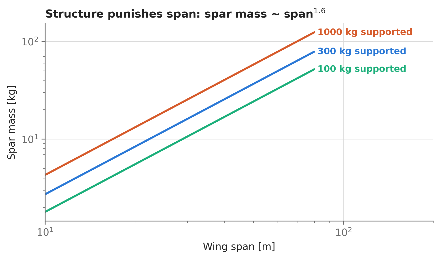
The second piece of intuition is structural. AeroSandbox ships a wing-spar mass model, aerosandbox.library.mass_structural.mass_wing_spar(), which is a closed-form fit (R² > 0.995) to a family of physics-based spar designs: each underlying design point is itself a beam-optimization problem — a cantilevered tube spar under an elliptical lift distribution, sized against strength and a tip-dihedral limit at the ultimate load factor. (The study that generated it lives in AeroSandbox/studies/MultiBoomSparMass_v2; the beam methods behind it are the subject of Chapter 9.) Figure 16.2 shows the fit: spar mass grows like span\(^{1.6}\), so doubling the span triples the spar mass, even before accounting for the extra weight it must then carry.

import _common
import matplotlib.pyplot as plt
from aerosandbox.library import mass_structural as structure

fig, ax = plt.subplots(figsize=(7, 3.6))
spans_plot = np.geomspace(10, 80, 100)
for m_supported, color in [(1000, _common.SERIES[3]), (300, _common.SERIES[0]),
                           (100, _common.SERIES[1])]:
    spar_mass = structure.mass_wing_spar(span=spans_plot, mass_supported=m_supported)
    ax.loglog(spans_plot, spar_mass, color=color)
    _common.label_line(ax, x=spans_plot[-1], y=spar_mass[-1],
                       text=f"{m_supported} kg supported", color=color, dx=2)
ax.set_xlim(10, 200)
ax.set_xlabel("Wing span [m]")
ax.set_ylabel("Spar mass [kg]")
ax.set_title("Structure punishes span: spar mass ~ span$^{1.6}$")
plt.show()

Figure 16.2: Wing spar mass vs. span, from mass_wing_spar() — a closed-form fit to a family of optimized cantilevered tube-spar designs. On these log-log axes the model is a straight line of slope ≈1.6: structure punishes span superlinearly. Curves shown for three values of supported (non-wing) mass.

These two scaling laws close a feedback loop that either converges or doesn’t: more battery → more weight → more wing → more drag and structure → more power → more battery. Whether that spiral converges to an airplane — and how big that airplane is — is exactly what the optimizer will tell us.

16.3 The sizing problem

We formulate the design as a single-design-point optimization: one cruise condition, flown identically day and night, with the day/night asymmetry captured entirely in the battery’s state of charge. (The real Dawn problem optimized the full 24-hour trajectory with ~150 collocation points and discovered altitude-cycling strategies; that extension uses the tools of Section 12.1, and we’ll note where it would attach.)

Table 16.1: Formulation of the solar HALE sizing problem.

Objective	minimize wing span \(b\)
Design variables	span \(b\), wing area \(S\), airspeed \(V\), altitude \(h\), gross mass \(m\), battery capacity \(E_\mathrm{batt}\), angle of attack \(\alpha\), tail boom length \(\ell\), wing rib count, and battery state-of-charge \(\mathrm{SoC}(t)\) at 97 points over the day — 106 variables total
Constraints	lift = weight; battery SoC dynamics (energy closure over 24 h, SoC within depth-of-discharge limits, periodic); airspeed ≥ 95th-percentile wind; altitude ≥ 60,000 ft; mass closure (gross mass ≥ sum of component masses)
Parameters	latitude, day of year, payload mass & power, battery technology

The disciplines couple exactly as in the Dawn design tool’s XDSM: the atmosphere feeds density to aerodynamics and propulsion; aerodynamics produces the drag that sets propulsion power; propulsion power plus payload power sets the electrical load on the power system, whose solar input depends on altitude; structures & weights turn geometry and gross mass into component masses; and two closure constraints — energy closure and mass closure — tie the loop shut. There is no nested “multidisciplinary analysis” iteration anywhere: as in Chapter 14, the couplings are just shared opti variables, and IPOPT converges the whole system simultaneously (the simultaneous analysis and design architecture).

A few modeling choices deserve explanation before you read the code:

• Stability is pinned by tail volume coefficients. At the conceptual level, fixing the horizontal and vertical tail volume coefficients (\(V_H = 0.45\), \(V_V = 0.02\), sailplane-typical values) is equivalent to fixing static margin — it sizes the tail surfaces as the wing and boom change. A proper neutral-point analysis via stability derivatives is shown in Section 7.4.
• The airfoil polar comes from NeuralFoil, live inside the optimization. We use the Drela DAE-11 (a low-Reynolds, high-lift section from the MIT Daedalus program) and query its lift and profile drag at the current \(\alpha\) and Reynolds number on every optimizer iteration, as in Section 6.1. The optimizer — not us — picks the operating \(c_\ell\), trading profile drag against induced drag and wing size.
• Battery dynamics are written as an inequality. The state of charge is allowed to increase by at most the net charging energy in each interval. This one-character trick (<= instead of ==) lets the optimizer shed surplus solar power at midday when the battery is full, without any explicit “dump load” logic. Shedding energy never helps the objective, so the constraint is tight whenever the energy actually matters. Note also how the constraint is written: multiplied through by battery_capacity rather than dividing by it. Dividing by a decision variable inside 96 constraints injects nasty \(1/x\) curvature; the multiplied form is merely bilinear, and in testing this reformulation alone cut typical solve iteration counts by several-fold (the lesson of Section 3.4, live in the field).
• Weights come from the AeroSandbox library. Wing secondary structure, tail surfaces, and boom use the Daedalus-derived correlations of Cruz (mass_hpa_wing, mass_hpa_stabilizer, mass_hpa_tail_boom); the spar uses mass_wing_spar (conservatively fed the full gross mass as supported mass); battery, motor, ESC, and MPPT masses come from propulsion_electric and power_solar. The wing rib count is a design variable — the model trades rib weight against leading-edge sheeting weight, a trade the library docstring explicitly invites you to optimize.
• Everything positive and scale-varying is log-transformed (log_transform=True), following Section 3.4: masses, areas, speeds, and battery capacity range over orders of magnitude across the sweeps we’ll run, and log-space keeps them positive and well-scaled.

16.4 The model

Here is the complete sizing tool. It’s a single function so that we can call it repeatedly for design sweeps; read it top to bottom — the section banners mirror the discipline map above.

from aerosandbox.library import (
    propulsion_electric as prop_elec,
    propulsion_propeller as prop_prop,
    mass_structural as structure,
    winds,
)

airfoil = asb.Airfoil("dae11")  # Drela DAE-11: low-Re, high-lift section


def size_solar_uav(
    latitude=35,                       # [deg] station-keeping latitude
    day_of_year=172,                   # June 21: summer solstice
    mass_payload=30,                   # [kg]
    power_payload=250,                 # [W] continuous
    min_altitude=18288,                # [m] (= 60,000 ft)
    battery_cell_specific_energy=400,  # [Wh/kg] at cell level
    n_timesteps=97,                    # points discretizing the 24 h cycle
    initial_guesses=None,              # dict; warm-start from a prior solve
):
    """Sizes a minimum-span solar-electric HALE UAV for perpetual flight
    at a single design point. Returns a dict of solved design quantities."""
    guess = {  # generic order-of-magnitude starting point
        "span": 40, "wing_area": 80, "airspeed": 30, "altitude": 20e3,
        "mass_total": 300, "battery_capacity": 250e6, "alpha": 4,
        "boom_length": 4, "n_ribs": 150,
    }
    guess.update(initial_guesses or {})

    ### Technology assumptions
    eta_prop, eta_motor, eta_esc = 0.85, 0.92, 0.97  # efficiencies [-]
    solar_cell_efficiency = 0.243      # SunPower C60-class cells [-]
    eta_solar_system = 0.90 * 0.96     # installation losses x MPPT [-]
    solar_margin = 0.95                # flat 5% energy-generation margin
    solar_area_fraction = 0.80         # fraction of wing covered by cells
    solar_areal_density = 0.45         # cells + encapsulation [kg/m^2]
    battery_pack_cell_fraction = 0.75  # cell mass / pack mass [-]
    max_depth_of_discharge = 0.85      # usable fraction of capacity [-]
    power_avionics = 50                # [W]
    g = 9.81                           # [m/s^2]

    opti = asb.Opti()

    ### Design variables
    span = opti.variable(init_guess=guess["span"], lower_bound=1)  # [m]
    wing_area = opti.variable(  # [m^2]
        init_guess=guess["wing_area"], log_transform=True)
    airspeed = opti.variable(  # [m/s]
        init_guess=guess["airspeed"], log_transform=True)
    altitude = opti.variable(  # [m]
        init_guess=guess["altitude"],
        lower_bound=min_altitude, upper_bound=30e3)
    mass_total = opti.variable(  # [kg]
        init_guess=guess["mass_total"], log_transform=True)
    battery_capacity = opti.variable(  # [J]
        init_guess=guess["battery_capacity"], log_transform=True)
    alpha = opti.variable(  # [deg]
        init_guess=guess["alpha"], lower_bound=-5, upper_bound=12)
    boom_length = opti.variable(  # [m]
        init_guess=guess["boom_length"], log_transform=True)
    n_ribs = opti.variable(  # [-]
        init_guess=guess["n_ribs"], lower_bound=10, log_transform=True)

    aspect_ratio = span**2 / wing_area
    mean_chord = wing_area / span

    ### Atmosphere + aerodynamics
    atmo = asb.Atmosphere(altitude=altitude)
    q = 0.5 * atmo.density() * airspeed**2  # dynamic pressure [Pa]
    Re = atmo.density() * airspeed * mean_chord / atmo.dynamic_viscosity()

    wing_aero = airfoil.get_aero_from_neuralfoil(  # sectional polar, live
        alpha=alpha, Re=Re, model_size="medium"
    )
    CL = wing_aero["CL"]
    opti.subject_to(mass_total * g == q * wing_area * CL)  # lift = weight

    # Tail sizing: fixed tail volume coefficients pin static stability.
    V_H, V_V = 0.45, 0.02
    S_hstab = V_H * wing_area * mean_chord / boom_length
    S_vstab = V_V * wing_area * span / boom_length

    drag = q * (
        wing_area * (
            wing_aero["CD"]                          # wing profile drag
            + CL**2 / (np.pi * 0.95 * aspect_ratio)  # induced drag, e = 0.95
        )
        + (S_hstab + S_vstab) * 0.010                # tail profile drag
        + 0.02                                       # payload pod drag area [m^2]
    )

    ### Propulsion + electrical loads
    power_shaft = drag * airspeed / eta_prop
    power_out = (power_shaft / (eta_motor * eta_esc)
                 + power_payload + power_avionics)   # total draw [W]
    power_rating = 2 * power_shaft  # installed power: margin for climb/gusts

    ### Solar input over one 24 h cycle (t = 0 at solar noon)
    time = np.linspace(0, 86400, n_timesteps)  # [s]
    solar_area = solar_area_fraction * wing_area
    power_in = solar.solar_flux(
        latitude=latitude, day_of_year=day_of_year, time=time, altitude=altitude,
    ) * solar_area * solar_cell_efficiency * eta_solar_system * solar_margin

    ### Battery energy accounting: the heart of the problem
    soc = opti.variable(  # battery state of charge over the day [-]
        init_guess=0.5, n_vars=n_timesteps,
        lower_bound=1 - max_depth_of_discharge, upper_bound=1,
    )
    net_power = power_in - power_out  # [W]
    opti.subject_to(  # inequality, so surplus solar power may be shed:
        battery_capacity * (soc[1:] - soc[:-1])
        <= (net_power[1:] + net_power[:-1]) / 2 * np.diff(time)
    )
    opti.subject_to(soc[-1] >= soc[0])  # diurnal energy closure

    ### Station-keeping: outfly the 95th-percentile wind
    wind_speed = winds.wind_speed_world_95(altitude, latitude, day_of_year)
    opti.subject_to(airspeed >= wind_speed)

    ### Mass buildup
    q_never_exceed = 2 * q
    mass_wing = structure.mass_wing_spar(     # primary structure (spar)
        span=span, mass_supported=mass_total,  # conservative: full gross mass
    ) + structure.mass_hpa_wing(              # secondary: Daedalus-derived
        span=span, chord=mean_chord, vehicle_mass=mass_total,
        n_ribs=n_ribs, t_over_c=0.128, include_spar=False,
    )
    mass_battery = prop_elec.mass_battery_pack(
        battery_capacity_Wh=battery_capacity / u.hour,
        battery_cell_specific_energy_Wh_kg=battery_cell_specific_energy,
        battery_pack_cell_fraction=battery_pack_cell_fraction,
    )
    tail_AR = 6  # assumed aspect ratio of tail surfaces
    masses = {
        "Battery pack": mass_battery,
        "Wing structure": mass_wing,
        "Payload": mass_payload,
        "Solar cells + MPPT": (
            solar_area * solar_areal_density
            + solar.mass_MPPT(power_in[0] / solar_margin)  # peak solar power
        ),
        "Pod structure": 0.10 * (mass_payload + mass_battery),
        "Tails + boom": (
            sum(
                structure.mass_hpa_stabilizer(
                    span=(tail_AR * S) ** 0.5, chord=(S / tail_AR) ** 0.5,
                    dynamic_pressure_at_manuever_speed=q_never_exceed,
                    n_ribs=(tail_AR * S) ** 0.5 / 0.20,  # one rib per 20 cm
                )
                for S in [S_hstab, S_vstab]
            )
            + structure.mass_hpa_tail_boom(
                length_tail_boom=boom_length + mean_chord,  # wing to tail
                dynamic_pressure_at_manuever_speed=q_never_exceed,
                mean_tail_surface_area=(S_hstab + S_vstab) / 2,
            )
        ),
        "Avionics": 5,
        "Motors + props + ESC": (
            2 * prop_elec.mass_motor_electric(max_power=power_rating / 2)
            + 2 * prop_prop.mass_hpa_propeller(diameter=2.5,
                                               max_power=power_rating / 2)
            + prop_elec.mass_ESC(max_power=power_rating)
        ),
    }
    opti.subject_to(mass_total >= sum(masses.values()))  # mass closure

    opti.minimize(span / 40)  # scaled to O(1)

    sol = opti.solve(verbose=False)
    return {
        "span": sol(span), "wing_area": sol(wing_area),
        "aspect_ratio": sol(aspect_ratio), "mass_total": sol(mass_total),
        "airspeed": sol(airspeed), "wind_speed": sol(wind_speed),
        "altitude": sol(altitude), "CL": sol(CL), "alpha": sol(alpha),
        "L_over_D": sol(mass_total * g / drag), "Re": sol(Re),
        "battery_capacity": sol(battery_capacity), "power_out": sol(power_out),
        "boom_length": sol(boom_length), "n_ribs": sol(n_ribs),
        "analysis_confidence": sol(wing_aero["analysis_confidence"]),
        "masses": {k: sol(v) for k, v in masses.items()},
        "time": time, "soc": sol(soc), "power_in": sol(power_in),
        "n_iterations": sol.stats()["iter_count"],
    }

Two closure constraints do the multidisciplinary work. The mass closure mass_total >= sum(masses.values()) is written as an inequality for solver robustness, but it behaves as an equality at the optimum: every spare kilogram of mass_total costs lift, power, and ultimately span, so the optimizer squeezes it tight. The energy closure soc[-1] >= soc[0] is the “flies forever” requirement — with the SoC bounds, it forces the battery, solar array, and power draw into mutual consistency.

16.5 The design point

Let’s size the baseline aircraft.

import time as timer

start = timer.time()
dp = size_solar_uav()
solve_time = timer.time() - start

print(f"Solved in {solve_time:.1f} s wall time "
      f"({dp['n_iterations']} IPOPT iterations).")
print(f"Minimum-span design: {dp['span']:.1f} m span, "
      f"{dp['mass_total']:.0f} kg gross mass.")

Solved in 3.0 s wall time (37 IPOPT iterations).
Minimum-span design: 28.7 m span, 229 kg gross mass.

The optimizer converges in seconds, from a generic initial guess, on a problem coupling six disciplines — this is the payoff of the differentiable, simultaneous formulation. Here’s the design it found, next to the published MIT Dawn baseline for reference:

Quantity	This chapter	MIT Dawn (published)
Wing span	28.7 m	39.9 m
Gross mass	229 kg	375 kg
Wing area	39.1 m²	67.9 m²
Aspect ratio	21.1	23.4
Wing loading	57.5 Pa	54.2 Pa
Cruise airspeed (true)	27.1 m/s	30.4 m/s
Cruise altitude	18.3 km	18.7–19.7 km
Cruise \(C_L\)	1.36	1.11
Cruise \(L/D\)	30.3	30.8
Wing Reynolds number	299k	383k
Battery capacity	38.5 kWh	75.4 kWh
Total electrical draw	2.95 kW	5.07 kW (peak)

The comparison is encouraging in exactly the way it should be. (Dawn’s baseline values here are from the program’s published conceptual design, as documented in Peter Sharpe’s MIT PhD thesis and the Dawn Design Tool.) The intensive quantities land close to the published Dawn values — wing loading within a few pascals, \(L/D\) within a few percent, cruise speed within a few m/s, and a cruise \(C_L\) in the same high-lift regime — because they’re set by the same physics: low-Reynolds airfoil performance, minimum-power flight, stratospheric density. The extensive quantities come out smaller, and each gap is traceable to a requirement we simplified: Dawn closes energy on August 31 (the end of a 6-week mission window, with 11.2 hours of night at this latitude versus our solstice-day 9.6), carries a payload that draws 500 W by day, must station-keep anywhere over the continental U.S. rather than at one benign latitude, and carries structural margins for gust loads and a full \(V\)–\(n\) envelope. Requirements, not physics, are what make solar airplanes big.

Note also analysis_confidence = 0.96 from NeuralFoil — worth checking whenever an optimizer is free to exploit an aerodynamic surrogate (Section 6.5).

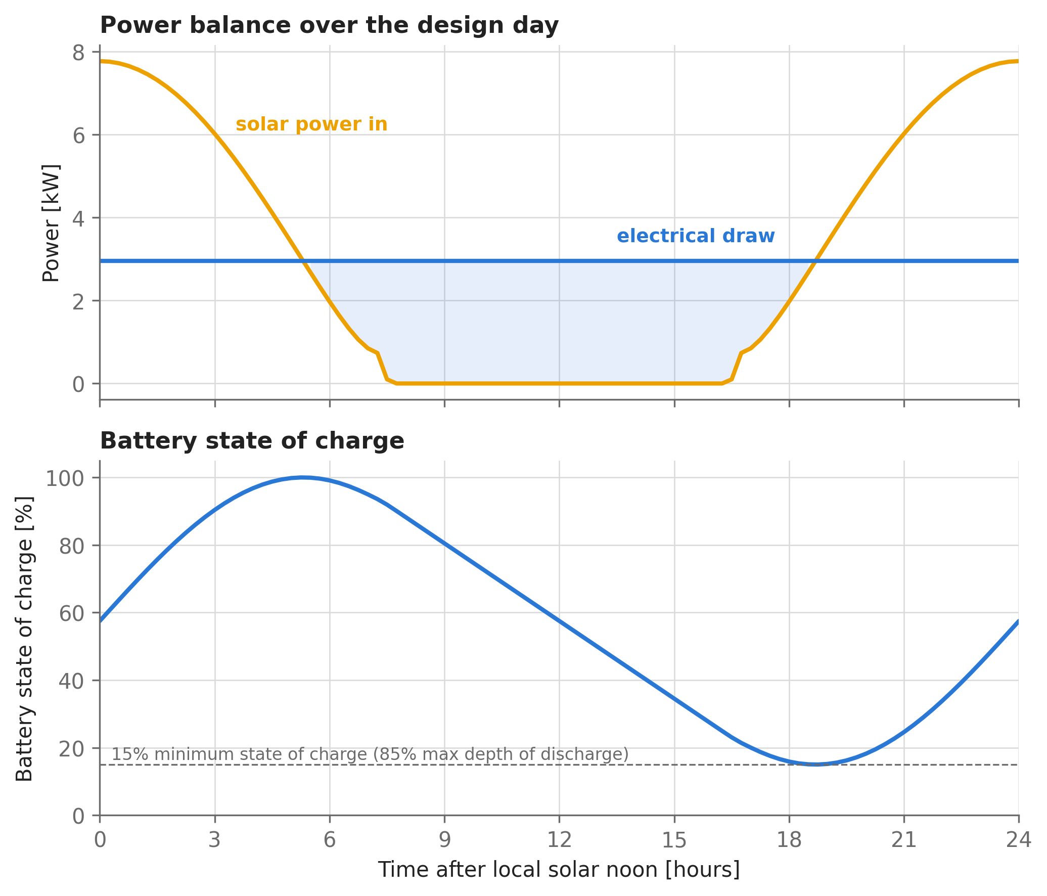
Figure 16.3 shows the day in the life of this aircraft that the optimizer implicitly planned:

import _common
import matplotlib.pyplot as plt

hours = dp["time"] / u.hour
fig, ax = plt.subplots(2, 1, figsize=(7, 6), sharex=True)

### Top: power in vs. power out
ax[0].plot(hours, dp["power_in"] / 1e3, color=_common.SERIES[2])
i_label = np.argmin(np.abs(hours - 3.3))  # anchor label to the curve at ~3.3 h
_common.label_line(ax[0], x=hours[i_label], y=dp["power_in"][i_label] / 1e3,
                   text="solar power in", color=_common.SERIES[2],
                   dx=0.3, dy=0.5)
ax[0].axhline(dp["power_out"] / 1e3, color=_common.SERIES[0], linewidth=2)
_common.label_line(ax[0], x=13.5, y=dp["power_out"] / 1e3,
                   text="electrical draw", color=_common.SERIES[0], dy=0.6)
ax[0].fill_between(
    hours, dp["power_in"] / 1e3, dp["power_out"] / 1e3,
    where=dp["power_in"] < dp["power_out"],
    color=_common.SERIES[0], alpha=0.12, linewidth=0,
)
ax[0].set_ylabel("Power [kW]")
ax[0].set_title("Power balance over the design day")

### Bottom: battery state of charge
ax[1].plot(hours, dp["soc"] * 100, color=_common.SERIES[0])
ax[1].axhline(15, color=_common.TEXT_SECONDARY, linewidth=0.8, linestyle="--")
ax[1].text(0.3, 16.5, "15% minimum state of charge (85% max depth of discharge)",
           color=_common.TEXT_SECONDARY, fontsize=8)
ax[1].set_xlim(0, 24)
ax[1].set_xticks(np.arange(0, 25, 3))
ax[1].set_ylim(0, 105)
ax[1].set_xlabel("Time after local solar noon [hours]")
ax[1].set_ylabel("Battery state of charge [%]")
ax[1].set_title("Battery state of charge")

plt.tight_layout()
plt.show()

Figure 16.3: The optimized design’s day, starting at solar noon. Top: solar power collected vs. total electrical draw. The morning surplus recharges the battery; the shaded gap is what the battery must bridge. Bottom: battery state of charge. The battery tops out just before the afternoon flux collapses, rides down through the night, and touches its 15% floor exactly at the dawn crossover — the energy-closure constraint is active, as a minimum-span design demands.

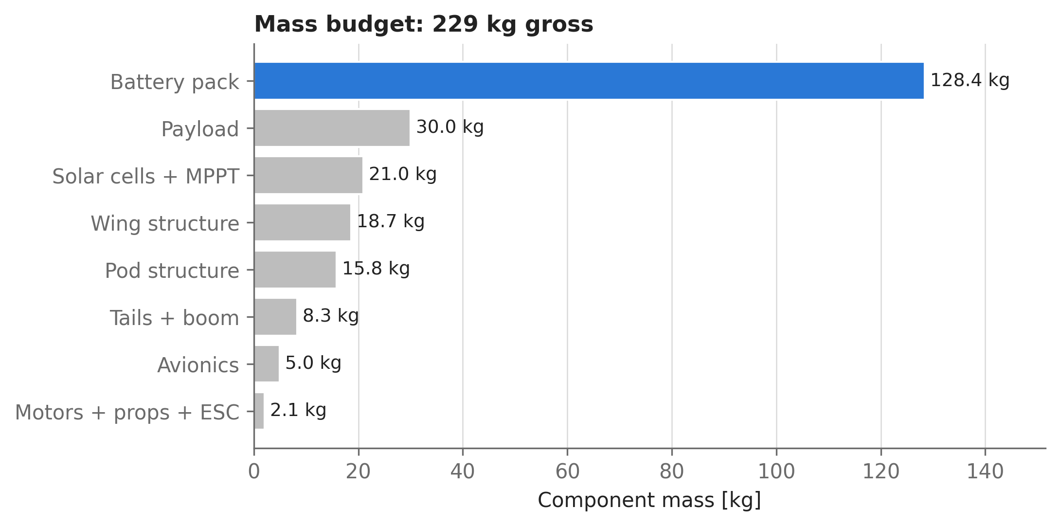
And Figure 16.4 shows where the mass went. The battery pack is 56% of gross mass — echoing the published Dawn breakdown, where the battery is nearly half the aircraft — while the payload, the entire point of the mission, is just 13%.

import _common
import matplotlib.pyplot as plt

items = sorted(dp["masses"].items(), key=lambda kv: kv[1])
names = [k for k, v in items]
values = np.array([v for k, v in items])
colors = [_common.SERIES[0] if k == "Battery pack" else "#bdbdbd"
          for k in names]

fig, ax = plt.subplots(figsize=(7, 3.6))
ax.barh(names, values, color=colors, edgecolor="white")
for i, v in enumerate(values):
    ax.text(v + 1, i, f"{v:.1f} kg", va="center", fontsize=9,
            color=_common.TEXT_PRIMARY)
ax.set_xlim(0, values.max() * 1.18)
ax.set_xlabel("Component mass [kg]")
ax.set_title(f"Mass budget: {dp['mass_total']:.0f} kg gross")
ax.grid(axis="y", visible=False)
plt.show()

Figure 16.4: Mass breakdown of the optimized design. Color marks the component that dominates the design problem: the battery. A solar HALE aircraft is best understood as a flying battery with a science instrument attached.

Three details of the solution are worth interrogating, because they show the optimizer reasoning rather than just filling in numbers:

• The altitude constraint is active: the aircraft flies at exactly 18.29 km, the 60,000 ft floor. Altitude buys slightly more solar flux but costs power as density falls, and at this latitude the 95th-percentile wind (19 m/s) is already below the min-power airspeed (27 m/s), so there’s no wind incentive to climb either. The optimizer parks on the bound.
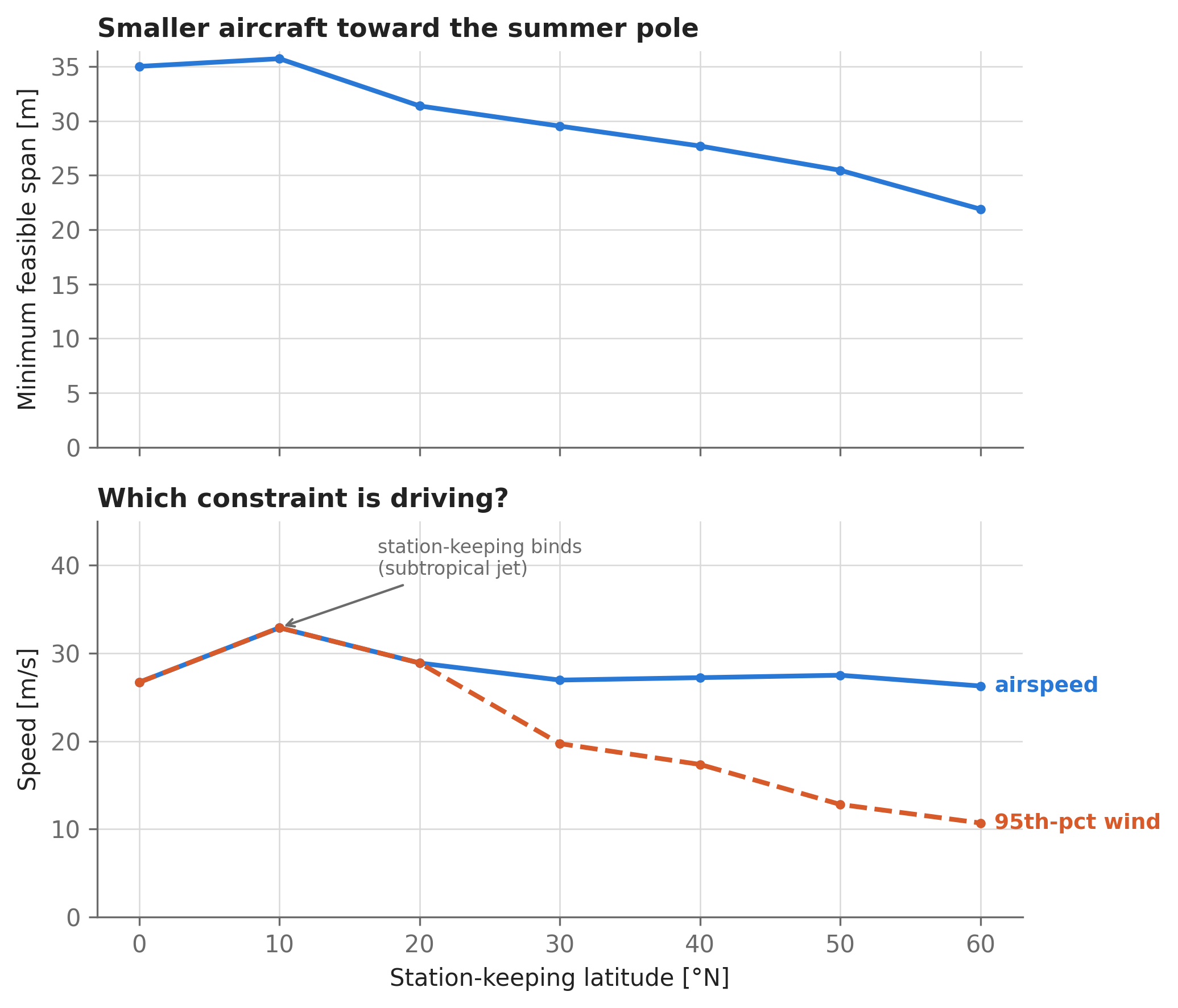
• The airspeed constraint is not active here — the aircraft flies its aerodynamic sweet spot, not the wind floor. We’ll see in the latitude sweep that this flips near the subtropical jet.
• The rib count lands at 115 ribs — a rib every 25 cm, right in the range of built Daedalus-class wings, from a variable that was free to be anything.

Since we discretized the day, we should verify the answer isn’t an artifact of the grid — the same refinement discipline as in Section 12.1:

dp_coarse = size_solar_uav(n_timesteps=49)
rel_change = abs(dp_coarse["span"] - dp["span"]) / dp["span"]
print(f"Halving the time resolution changes the span by {rel_change:.2%}.")

Halving the time resolution changes the span by 0.12%.

16.6 Interrogating the design space

A sizing function that solves in seconds is a question-answering machine. The Dawn program’s most valuable early artifact was not any single design, but a map: 2,400 optimized aircraft across a latitude–season grid, answering “how big an airplane does this mission need?” in one figure. We’ll reproduce two 1-D slices of that map.

Since each sweep point is a nearby variant of the baseline, we warm-start every solve from the baseline solution — re-centering the initial guesses on a known-good design cuts iterations and makes far-from-baseline points solve much more reliably (more on sweep strategies in Section 5.5):

warm = {
    k: dp[k]
    for k in ["span", "wing_area", "airspeed", "altitude", "mass_total",
              "battery_capacity", "alpha", "boom_length", "n_ribs"]
}

Where can a small aircraft fly? Sweep latitude, re-optimizing the whole aircraft at each point:

latitudes = np.arange(0, 61, 10)
lat_designs = [
    size_solar_uav(latitude=lat, initial_guesses=warm) for lat in latitudes
]

import _common
import matplotlib.pyplot as plt

spans = np.array([d["span"] for d in lat_designs])
speeds = np.array([d["airspeed"] for d in lat_designs])
wind = np.array([d["wind_speed"] for d in lat_designs])

fig, ax = plt.subplots(2, 1, figsize=(7, 6), sharex=True)

ax[0].plot(latitudes, spans, ".-", color=_common.SERIES[0])
ax[0].set_ylabel("Minimum feasible span [m]")
ax[0].set_title("Smaller aircraft toward the summer pole")
ax[0].set_ylim(bottom=0)

ax[1].plot(latitudes, speeds, ".-", color=_common.SERIES[0])
_common.label_line(ax[1], x=latitudes[-1], y=speeds[-1], text="airspeed",
                   color=_common.SERIES[0], dx=1)
ax[1].plot(latitudes, wind, ".--", color=_common.SERIES[3])
_common.label_line(ax[1], x=latitudes[-1], y=wind[-1],
                   text="95th-pct wind", color=_common.SERIES[3], dx=1)
ax[1].annotate("station-keeping binds\n(subtropical jet)",
               xy=(10, wind[1]), xytext=(17, wind[1] + 6),
               color=_common.TEXT_SECONDARY, fontsize=8,
               arrowprops=dict(arrowstyle="->", color=_common.TEXT_SECONDARY))
ax[1].set_xlabel("Station-keeping latitude [°N]")
ax[1].set_ylabel("Speed [m/s]")
ax[1].set_title("Which constraint is driving?")
ax[1].set_ylim(0, 45)

plt.tight_layout()
plt.show()

Figure 16.5: Re-optimized minimum-span designs vs. station-keeping latitude (northern-hemisphere summer solstice). Top: required span. Bottom: why — near the subtropical jet the station-keeping constraint binds (airspeed pinned to the 95th-percentile wind), while toward the pole the shortening night shrinks the battery and the whole aircraft.

Two competing effects shape Figure 16.5. Toward the pole, summer nights shorten, the battery shrinks, and with it the entire aircraft — at 60° N the minimum span is 22 m versus 35 m at the equator, despite weaker peak sun. This is the “solar panels are light, batteries are heavy” asymmetry made visible, and it’s why the Dawn studies found Arctic summer missions surprisingly easy. But equatorward of about 25° N, the subtropical jet keeps the 95th-percentile wind above the aircraft’s preferred loiter speed: the bottom panel shows airspeed pinned to the wind line there (worst near the jet’s core around 10° N), and the aircraft must grow to carry the extra propulsive power. The design driver changes identity across the sweep — exactly the kind of insight a one-point design study can’t give you. (Remember these are solstice numbers: run the same sweep with day_of_year=355 and the polar advantage reverses catastrophically, as Figure 16.1 forewarned.)

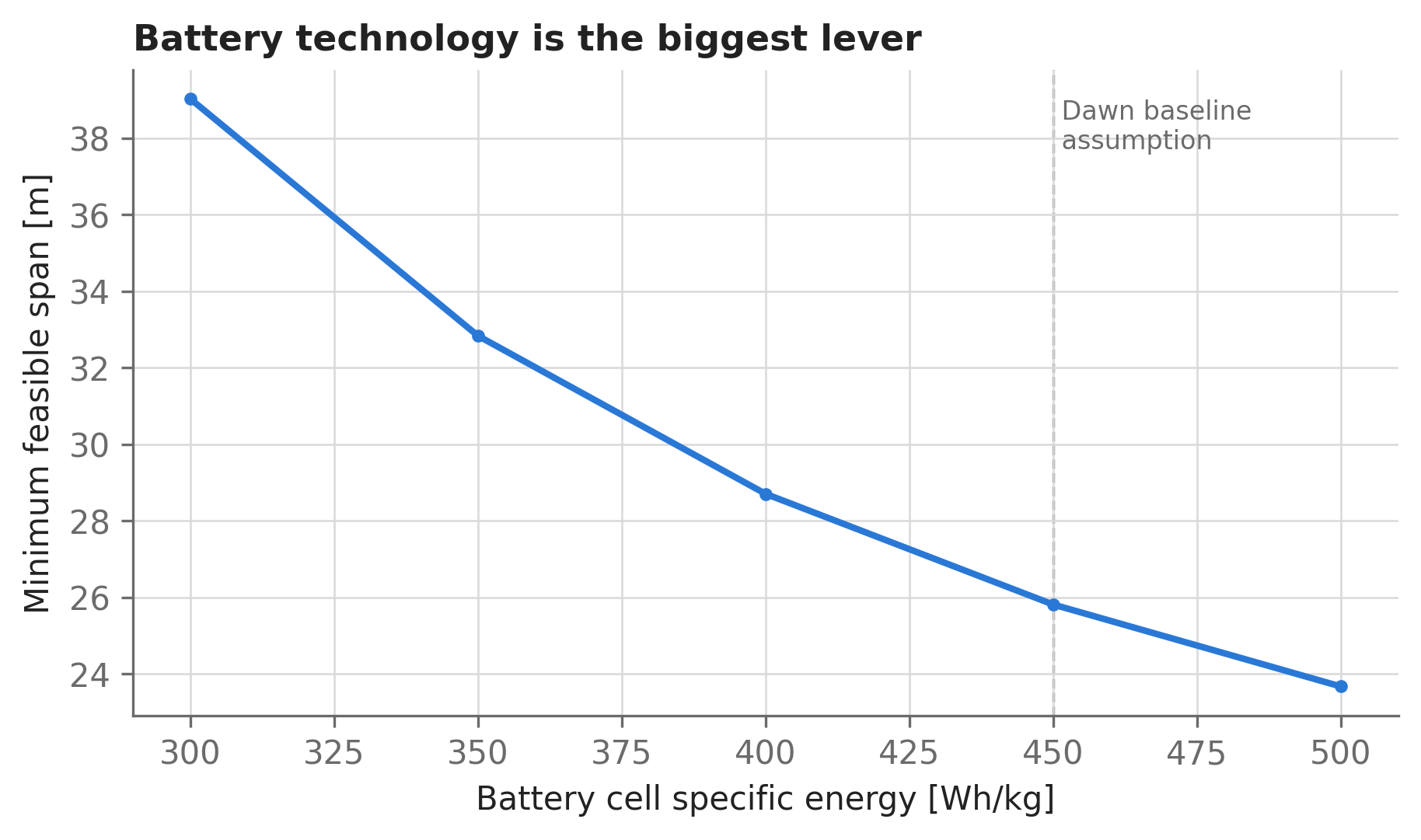
How much does battery technology matter? Battery cell specific energy is the most consequential technology assumption in the model:

cell_energies = np.arange(300, 501, 50)  # [Wh/kg]
batt_designs = [
    size_solar_uav(battery_cell_specific_energy=e, initial_guesses=warm)
    for e in cell_energies
]

import _common
import matplotlib.pyplot as plt

batt_spans = np.array([d["span"] for d in batt_designs])

fig, ax = plt.subplots(figsize=(7, 3.6))
ax.plot(cell_energies, batt_spans, ".-", color=_common.SERIES[0])
ax.axvline(450, color=_common.TEXT_SECONDARY, linewidth=0.8, linestyle="--",
           zorder=0)
ax.text(450, batt_spans.max(), " Dawn baseline\n assumption",
        color=_common.TEXT_SECONDARY, va="top", fontsize=8)
ax.set_xlabel("Battery cell specific energy [Wh/kg]")
ax.set_ylabel("Minimum feasible span [m]")
ax.set_title("Battery technology is the biggest lever")
plt.show()

Figure 16.6: Minimum feasible span vs. assumed battery cell specific energy, all else fixed. The Dawn program’s baseline assumption of 450 Wh/kg cells (silicon-anode / lithium-sulfur class) is marked. Battery technology is the single biggest lever in the entire problem.

Going from 300 to 500 Wh/kg cells shrinks the airplane from 39 m to 24 m of span — a 39% reduction (roughly 8 cm of wingspan per Wh/kg), worth more than most aerodynamic refinements combined. Sensitivity information like this is what design optimization is for: it tells you where to spend engineering effort (or R&D dollars) before you commit to hardware. For first-order sensitivities of a solved problem, you don’t even need a sweep — the Lagrange duals give them for free, as shown in Section 11.5.

16.7 What this model leaves out

About a hundred lines of model buys the right first-order answers, but be honest with yourself (and your stakeholders) about the simplifications before trusting it further:

• Single design point, not a trajectory. The aircraft flies one speed at one altitude, day and night. The full Dawn formulation optimizes a 24-hour collocated trajectory and discovers altitude cycling — climbing on afternoon solar surplus and gliding down overnight, using gravity as a second battery. That version bolts the machinery of Section 12.1 and Section 13.1 onto exactly this energy model.
• Solstice sizing. We sized on the easiest day of the year. A real mission must close energy on the worst day of its window (Dawn’s closure day was the end of its six-week mission), and the seasonality panel of Figure 16.1 shows how punishing that can be.
• Horizontal-panel solar model. Real wings have camber, dihedral, and bank; cells see the sun off-normal, and heading matters at dawn and dusk. solar_flux() accepts panel tilt and azimuth angles if you want to model this.
• Frozen efficiencies. Propeller, motor, and ESC efficiencies are constants here; the library’s motor_electric_performance() and propeller_shaft_power_from_thrust() support physics-based, operating-point-dependent versions.
• Statistical structures at HPA scale. The Daedalus-heritage weight correlations are extrapolated to a heavier, faster aircraft, the spar model conservatively carries full gross mass, and there is no gust-load or aeroelastic analysis — the very failure mode that motivated the min-span objective. A real program graduates to beam models (Chapter 9) and aeroelastic checks (Chapter 14).

Each of these is an upgrade within the same formulation — add variables, swap a model, tighten a constraint, re-solve. None requires restructuring the code, which is the quiet superpower of writing sizing problems this way.

16.8 Where to go next

• Section 12.1 shows the trajectory-optimization machinery (collocation, constrain_derivative) needed to turn this single-point sizing into a full 24-hour mission optimization with altitude cycling.
• Chapter 14 dives into the coupled aerostructural analysis that would replace this chapter’s statistical wing-weight models.
• Section 16.1 applies the same closure-constraint sizing pattern to a conventional transport aircraft — comparing the two chapters side-by-side is a good way to see what’s universal about the method.

For the full-fidelity version of this problem — mission-space maps over latitude and season, trajectory optimization, and the models behind the flight-proven Dawn aircraft — see the open-source Dawn Design Tool and the solar-aircraft design study in Peter Sharpe’s MIT PhD thesis.