import aerosandbox as asb
import aerosandbox.numpy as np

wing_airfoil = asb.Airfoil("sd7037")
tail_airfoil = asb.Airfoil("naca0010")

airplane = asb.Airplane(
    name="Peter's Glider",
    xyz_ref=[0, 0, 0],  # CG location; also the moment reference point
    wings=[
        asb.Wing(
            name="Main Wing",
            symmetric=True,
            xsecs=[
                asb.WingXSec(  # Root
                    xyz_le=[0, 0, 0],
                    chord=0.18,
                    twist=2,  # deg
                    airfoil=wing_airfoil,
                ),
                asb.WingXSec(  # Mid
                    xyz_le=[0.01, 0.5, 0],
                    chord=0.16,
                    twist=0,
                    airfoil=wing_airfoil,
                ),
                asb.WingXSec(  # Tip
                    xyz_le=[0.08, 1, 0.1],
                    chord=0.08,
                    twist=-2,
                    airfoil=wing_airfoil,
                ),
            ],
        ),
        asb.Wing(
            name="Horizontal Stabilizer",
            symmetric=True,
            xsecs=[
                asb.WingXSec(  # Root
                    xyz_le=[0, 0, 0],
                    chord=0.1,
                    twist=-10,
                    airfoil=tail_airfoil,
                    control_surfaces=[
                        asb.ControlSurface(
                            name="Elevator",
                            symmetric=True,  # Deflects together on both sides
                            hinge_point=0.75,  # Hinge at 75% chord
                        )
                    ],
                ),
                asb.WingXSec(  # Tip
                    xyz_le=[0.02, 0.17, 0],
                    chord=0.08,
                    twist=-10,
                    airfoil=tail_airfoil,
                ),
            ],
        ).translate([0.6, 0, 0.06]),
        asb.Wing(
            name="Vertical Stabilizer",
            symmetric=False,
            xsecs=[
                asb.WingXSec(
                    xyz_le=[0, 0, 0],
                    chord=0.1,
                    airfoil=tail_airfoil,
                ),
                asb.WingXSec(
                    xyz_le=[0.04, 0, 0.15],
                    chord=0.06,
                    airfoil=tail_airfoil,
                ),
            ],
        ).translate([0.6, 0, 0.07]),
    ],
    fuselages=[
        asb.Fuselage(
            name="Fuselage",
            xsecs=[
                asb.FuselageXSec(
                    xyz_c=[0.8 * xi - 0.1, 0, 0.1 * xi - 0.03],
                    radius=0.6 * asb.Airfoil("dae51").local_thickness(x_over_c=xi),
                )
                for xi in np.cosspace(0, 1, 30)
            ],
        )
    ],
)7 Aircraft Aerodynamics
You have an airplane geometry. Now you need forces and moments: how much lift at this angle of attack, how much drag at that cruise condition, whether the airplane is stable, and how all of that changes as the optimizer morphs the design. This chapter covers AeroSandbox’s built-in 3D aerodynamics analyses — what each one models, what each one costs, and how much to trust them. You will learn to run the same airplane through four solvers of increasing fidelity, extract stability derivatives, do a first aerodynamic shape optimization, and finally check all four methods against wind-tunnel data on a swept flying wing.
Every analysis here shares one interface: construct it from an asb.Airplane (Chapter 5) and an asb.OperatingPoint, call .run(), and get back a dictionary of forces, moments, and nondimensional coefficients with identical keys. Because the methods are interchangeable, you can prototype a design study with the fastest one and swap in a higher-fidelity one with a two-line change. And because every method is written in aerosandbox.numpy, each one is automatically differentiable — any of them can sit inside an asb.Opti problem as a design constraint.
7.1 The fidelity ladder
There is no single “best” aerodynamics model — only the right tool for the current design question. AeroSandbox gives you a ladder:
| Method | Class | Physics | Viscous? | Valid envelope | Relative cost |
|---|---|---|---|---|---|
| Component buildup | asb.AeroBuildup |
DATCOM-style analytic + empirical buildup, incl. fuselages | Yes | Any \(\alpha, \beta\) (±180°), subsonic through supersonic (reduced accuracy transonic) | Fastest; vectorizes over operating points |
| Vortex lattice | asb.VortexLatticeMethod |
3D lifting-surface potential flow | No | Attached flow, small-ish angles | Fast; scales with panel count |
| Lifting line | asb.LiftingLine |
Spanwise horseshoe-vortex system + NeuralFoil 2D viscous data | Yes | Attached flow, moderate angles | Fast |
| Nonlinear lifting line | asb.NonlinearLiftingLine |
Same, but circulation solved consistently with nonlinear 2D polars (implicit solve) | Yes | Attached flow, into early stall | Slowest (iterative solve) |
A good default workflow: use AeroBuildup for design-space exploration and full-envelope work (it is the only method here that models fuselage aerodynamics and remains well-behaved at extreme attitudes), then spot-check the converged design with the vortex lattice or lifting-line methods — or with external codes like AVL and XFoil (Section 18.1).
7.2 The running example
Concrete first: we need an airplane. Here is a small RC-glider-class aircraft — a main wing, tail surfaces (with an elevator on the horizontal stabilizer), and a streamlined fuselage. The geometry classes themselves are covered in Chapter 5; skim the code and note only that distances are in meters and angles in degrees.
airplane.draw_three_view()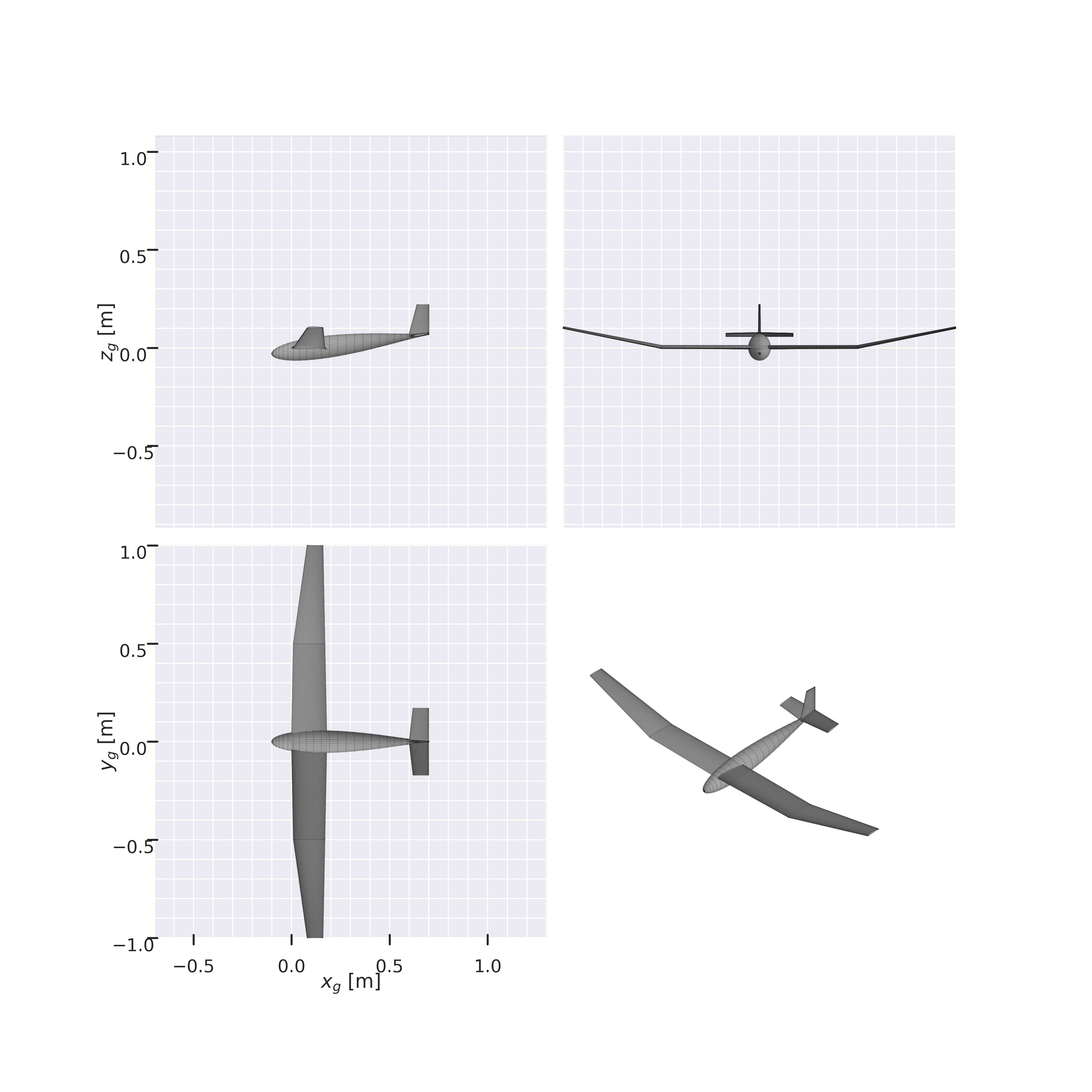
airplane.draw_three_view().
array([[<Axes3D: zlabel='$z_g$ [m]'>, <Axes3D: >],
       [<Axes3D: xlabel='$x_g$ [m]', ylabel='$y_g$ [m]'>, <Axes3D: >]],
dtype=object)<module '_common' from '/tmp/claude-1000/-home-psharpe-gh-AeroSandbox/1ccf6b40-3256-4f8d-9484-ebe00c7e55db/scratchpad/book-staging/_common.py'>7.3 AeroBuildup: the workhorse
asb.AeroBuildup computes forces and moments the way a classical conceptual-design workbook does: component by component, combining analytic theory (lifting-surface slopes, slender-body theory) with empirical corrections for viscous and compressible effects. Its formulation is heavily inspired by the USAF Digital DATCOM, and many submodels are shared with it. Two properties make it the workhorse of this chapter:
- It works everywhere. It returns finite, smoothly-varying answers across all 360° of angle of attack and sideslip, at arbitrary angular rates, from low subsonic through supersonic. (Accuracy degrades far from normal flight — an answer at \(\alpha = 90°\) is order-of-magnitude correct, not precise — but it never explodes, which is exactly what an optimizer crawling through bad intermediate designs needs.)
- It is fast and vectorized. Analyzing thousands of operating points in a single call costs milliseconds per point, as we will measure below.
7.3.1 A single operating point
An analysis takes the airplane plus an asb.OperatingPoint describing the flight condition — velocity, altitude (via an asb.Atmosphere), \(\alpha\), \(\beta\), and body rates \(p, q, r\):
op_point = asb.OperatingPoint(
    velocity=10,  # m/s
    alpha=5,  # deg
)

aero = asb.AeroBuildup(
    airplane=airplane,
    op_point=op_point,
).run()


def scalar(x):
    """Collapse a size-1 array to a plain float, for printing."""
    return float(np.ravel(x)[0])


for key in ["L", "D", "CL", "CD", "Cm"]:
    print(f"{key:>2} = {scalar(aero[key]):8.4f}")
L = 14.1459
D = 0.7256
CL = 0.7899
CD = 0.0405
Cm = -0.2177At 10 m/s and \(\alpha = 5°\), the glider makes 14.1 N of lift against 0.73 N of drag — a lift-to-drag ratio of 19.5.
The returned dictionary contains much more than these five entries. Forces F and moments M come as \([x, y, z]\) vectors in three frames, distinguished by suffix:
| Frame | Keys | Orientation |
|---|---|---|
| Geometry | F_g, M_g |
\(+x\) aft, \(+y\) out the right wing, \(+z\) up — same frame the geometry is defined in |
| Body | F_b, M_b |
\(+x\) out the nose, \(+y\) out the right wing, \(+z\) down |
| Wind | F_w, M_w |
\(+x\) along the flight velocity (into the relative wind), \(+z\) down |
The scalar entries are breakouts of these vectors: lift L, drag D, and sideforce Y (wind axes, with \(L = -F_{w,z}\) and \(D = -F_{w,x}\)); rolling/pitching/yawing moments l_b, m_b, n_b (body axes); and their nondimensional counterparts CL, CD, CY, Cl, Cm, Cn. Coefficients are normalized by airplane.s_ref, c_ref, and b_ref, which you can set explicitly or let AeroSandbox derive from the first wing. Moments are taken about xyz_ref — by default the airplane’s xyz_ref, so make sure that point is where you think your CG is.
7.3.2 Polars: vectorizing over operating points
AeroBuildup accepts array-valued operating points, so sweeping \(\alpha\) is one call, not a loop. Let’s measure how fast:
import time

alpha = np.linspace(-15, 15, 300)

t_start = time.time()
aero = asb.AeroBuildup(
    airplane=airplane,
    op_point=asb.OperatingPoint(velocity=10, alpha=alpha),
).run()
t_sweep = time.time() - t_start

print(f"{len(alpha)} operating points analyzed in {t_sweep * 1e3:.0f} ms "
      f"({t_sweep / len(alpha) * 1e3:.1f} ms per point)")
300 operating points analyzed in 565 ms (1.9 ms per point)That speed — about 2 ms per operating point for a complete airplane, viscous drag and all, with the per-point cost falling further for larger batches — is what makes AeroBuildup usable inside optimization loops and mission simulations. The resulting polars:
import _common  # book-wide plot style
import matplotlib.pyplot as plt

fig, ax = plt.subplots(4, 1, figsize=(7, 9.5), sharex=True)

ax[0].plot(alpha, aero["CL"], color=_common.SERIES[0])
ax[0].set_ylabel("$C_L$ [-]")
ax[0].set_title("Lift grows linearly, then softens toward stall")

ax[1].plot(alpha, aero["CD"], color=_common.SERIES[0])
ax[1].set_ylabel("$C_D$ [-]")
ax[1].set_ylim(bottom=0)
ax[1].set_title("Drag: friction floor plus induced-drag parabola")

ax[2].plot(alpha, aero["Cm"], color=_common.SERIES[0])
ax[2].axhline(0, color=_common.TEXT_SECONDARY, linewidth=0.8, linestyle="--")
ax[2].set_ylabel("$C_m$ [-]")
ax[2].set_title("Pitching moment: negative slope = statically stable")

ax[3].plot(alpha, aero["CL"] / aero["CD"], color=_common.SERIES[0])
ax[3].set_ylabel("$C_L/C_D$ [-]")
ax[3].set_xlabel(r"Angle of attack $\alpha$ [deg]")
ax[3].set_title("Aerodynamic efficiency peaks at a moderate angle of attack")

plt.tight_layout()
plt.show()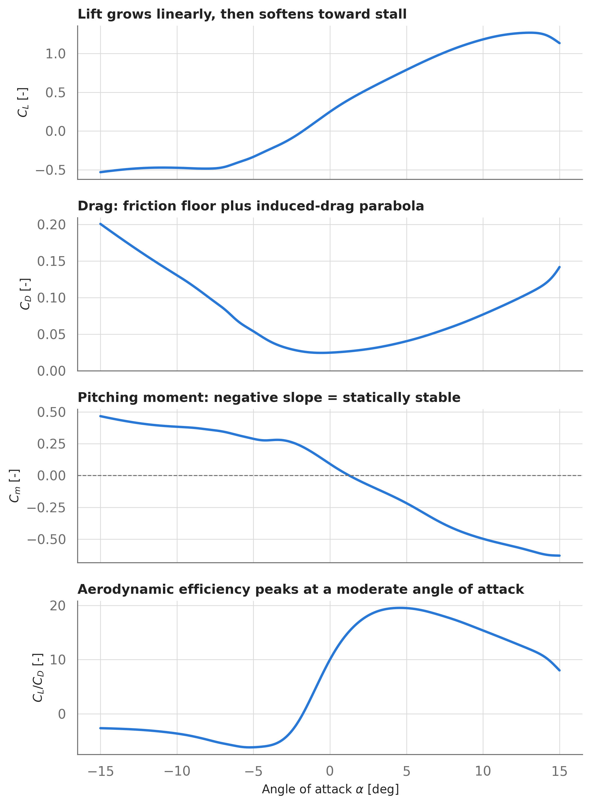
AeroBuildup call: lift, drag, pitching moment, and aerodynamic efficiency versus angle of attack.
Reading Figure 7.2 like an aerodynamicist: the lift curve is linear in the attached-flow regime with softening at the extremes; drag has a friction-dominated bucket near zero lift and grows quadratically with lift (induced drag); the pitching-moment slope is negative, so the airplane is statically stable in pitch; and efficiency peaks at \(L/D\) = 19.5 around \(\alpha\) = 4.6°.
7.3.3 The full envelope: any \(\alpha\), any \(\beta\)
Most aerodynamics tools quietly assume small angles. AeroBuildup does not — you can ask for the whole \((\alpha, \beta)\) envelope, which matters for spin analysis, high-angle trajectory simulation (e.g., rocket or re-entry-vehicle work), and making sure an optimizer can recover from absurd intermediate iterates. Here is the glider’s lift coefficient over ±90° in both angles — about 3,700 operating points, again in one vectorized call:
import _common
import matplotlib.pyplot as plt
from matplotlib.patches import Rectangle

Beta, Alpha = np.meshgrid(np.linspace(-90, 90, 61), np.linspace(-90, 90, 61))

aero_grid = asb.AeroBuildup(
    airplane=airplane,
    op_point=asb.OperatingPoint(
        velocity=10,
        alpha=Alpha.flatten(),
        beta=Beta.flatten(),
    ),
).run()

CL_grid = aero_grid["CL"].reshape(Alpha.shape)

fig, ax = plt.subplots(figsize=(7, 5.8))
vmax = np.max(np.abs(CL_grid))
cf = ax.contourf(Beta, Alpha, CL_grid, levels=21, cmap="RdBu_r",
                 vmin=-vmax, vmax=vmax, alpha=0.85)
cs = ax.contour(Beta, Alpha, CL_grid, levels=11, colors="white", linewidths=0.7)
ax.clabel(cs, fontsize=7, fmt="%.1f")
fig.colorbar(cf, label="Lift coefficient $C_L$ [-]")

ax.add_patch(Rectangle((-10, -15), 20, 30, fill=False,
                       edgecolor=_common.TEXT_PRIMARY, linewidth=1.2))
ax.annotate("conventional-analysis\nenvelope", xy=(12, -14),
            fontsize=8, color=_common.TEXT_PRIMARY, va="top")

ax.set_xlabel(r"Sideslip angle $\beta$ [deg]")
ax.set_ylabel(r"Angle of attack $\alpha$ [deg]")
ax.set_aspect("equal")
plt.show()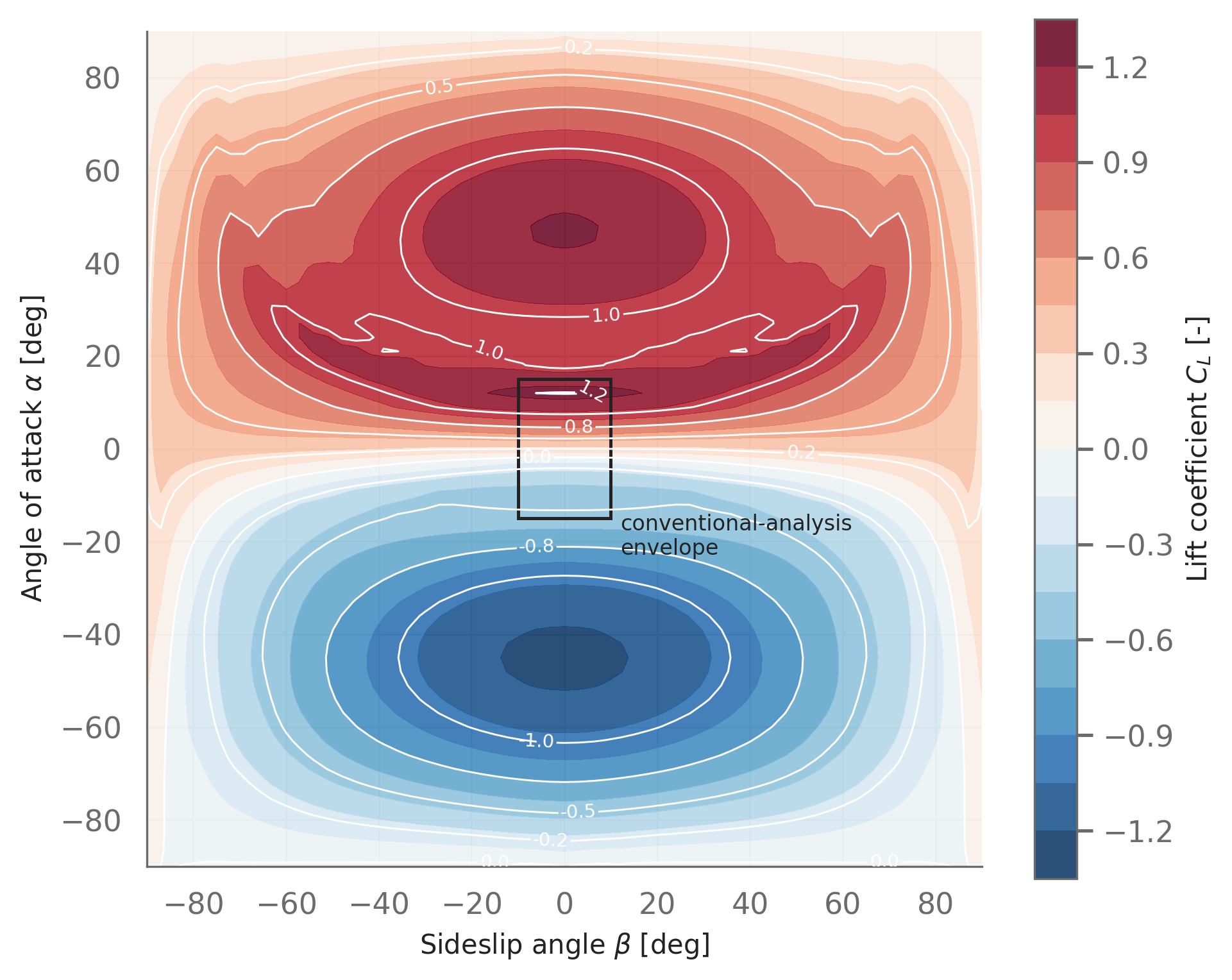
7.3.4 Control surfaces and trim
AeroBuildup also models control-surface deflections. We declared an asb.ControlSurface named "Elevator" on the horizontal stabilizer back in Section 7.2; airplane.with_control_deflections() returns a copy of the airplane with a deflection applied (positive = trailing edge down, by convention). Sweeping the elevator shifts the pitching-moment curve, which moves the trim point — the angle of attack where \(C_m = 0\) and the airplane is in pitch equilibrium:
import _common
import matplotlib.pyplot as plt

alpha_trim_sweep = np.linspace(-8, 12, 60)
deflections = [-6, -3, 0, 3, 6]  # deg
alpha_trims = []

fig, ax = plt.subplots(figsize=(7, 4.5))
for i, deflection in enumerate(deflections):
    aero_defl = asb.AeroBuildup(
        airplane=airplane.with_control_deflections({"Elevator": deflection}),
        op_point=asb.OperatingPoint(velocity=10, alpha=alpha_trim_sweep),
    ).run()

    # Trim: interpolate for the alpha where Cm crosses zero.
    # (Cm decreases with alpha, so flip the arrays for np.interp.)
    alpha_trim = np.interp(0, aero_defl["Cm"][::-1], alpha_trim_sweep[::-1])
    alpha_trims.append(alpha_trim)

    color = _common.SERIES[i]
    ax.plot(alpha_trim_sweep, aero_defl["Cm"], color=color)
    ax.plot(alpha_trim, 0, "o", color=color, markersize=6, zorder=4)
    _common.label_line(
        ax, alpha_trim_sweep[-1], aero_defl["Cm"][-1],
        rf"$\delta_e = {deflection:+d}°$", color, dx=0.3,
    )

ax.axhline(0, color=_common.TEXT_SECONDARY, linewidth=0.8, linestyle="--")
ax.set_xlabel(r"Angle of attack $\alpha$ [deg]")
ax.set_ylabel("Pitching moment coefficient $C_m$ [-]")
ax.set_xlim(right=17)  # room for the direct labels
plt.show()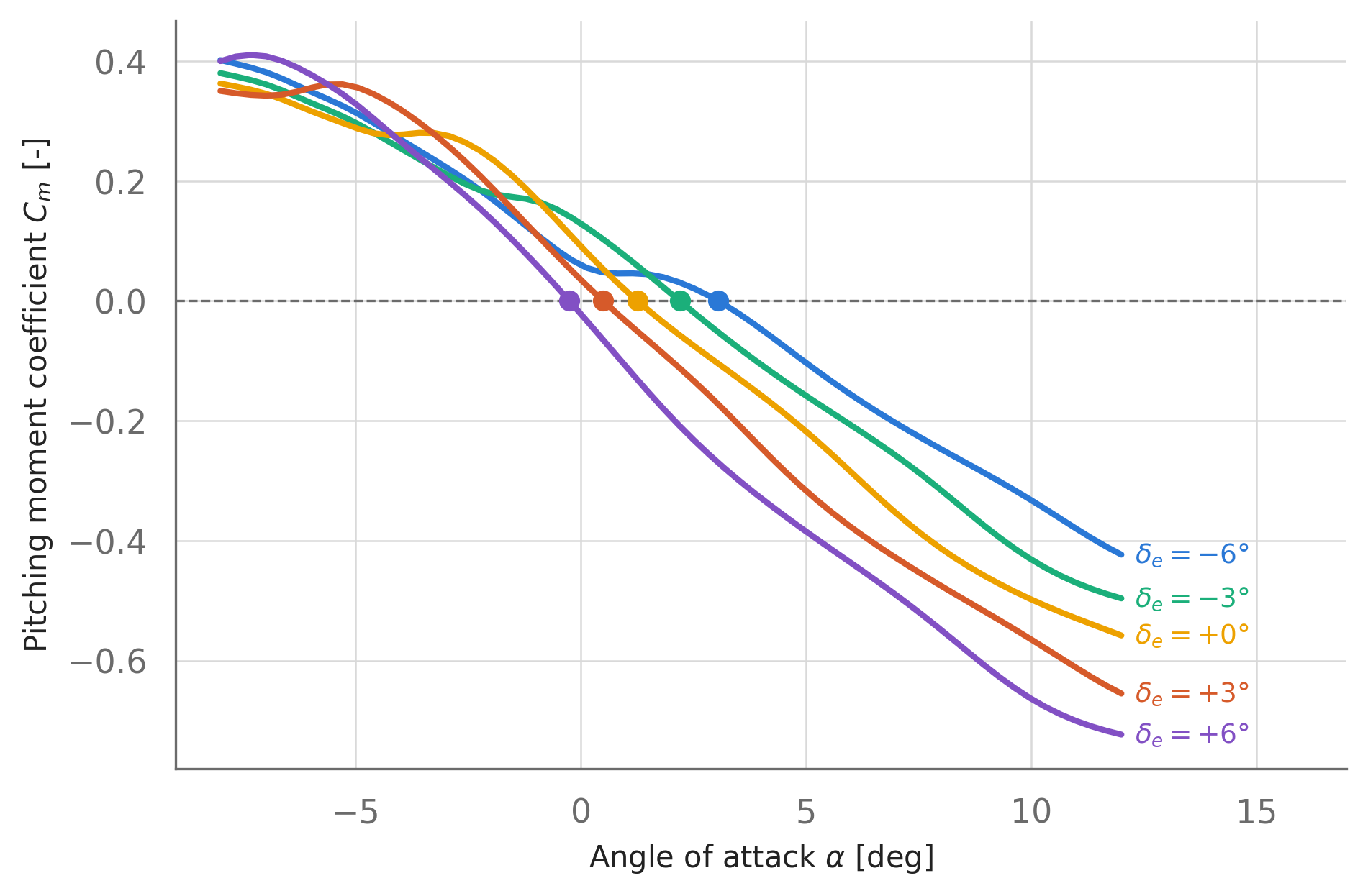
Each degree of down-elevator retrims the glider about 0.28° lower in angle of attack over this range — the kind of control-authority number you need when sizing tail surfaces.
7.4 Stability derivatives
Static stability analysis needs the derivatives of forces and moments with respect to flight condition — quantities like \(C_{m_\alpha}\) (pitch stiffness) and \(C_{n_\beta}\) (weathercock stability). Because every AeroSandbox model is automatically differentiable, you don’t need finite-difference sweeps: run_with_stability_derivatives() returns exact derivatives alongside the baseline results. (This method exists on AeroBuildup, VortexLatticeMethod, and LiftingLine alike.)
derivs = asb.AeroBuildup(
    airplane=airplane,
    op_point=asb.OperatingPoint(velocity=10, alpha=5),
).run_with_stability_derivatives()  # computes d/d{alpha, beta, p, q, r}

for key in ["CLa", "Cma", "Cmq", "Clb", "Clp", "Cnb", "Cnr", "x_np"]:
    print(f"{key:>4} = {scalar(derivs[key]):+8.4f}")
CLa = +5.5248
Cma = -3.6760
Cmq = -19.0596
Clb = -0.1701
Clp = -0.7000
Cnb = -0.0246
Cnr = -0.0158
x_np = +0.1005The key entries, and how to read their signs:
AeroBuildup.
| Derivative | Value | Meaning | Stable sign |
|---|---|---|---|
| \(C_{L_\alpha}\) | +5.52 /rad | Lift-curve slope | — |
| \(C_{m_\alpha}\) | -3.68 /rad | Pitch stiffness | negative |
| \(C_{m_q}\) | -19.06 /rad | Pitch damping | negative |
| \(C_{l_\beta}\) | -0.170 /rad | Dihedral effect (roll due to sideslip) | negative |
| \(C_{l_p}\) | -0.70 /rad | Roll damping | negative |
| \(C_{n_\beta}\) | -0.025 /rad | Weathercock (yaw) stability | positive |
| \(C_{n_r}\) | -0.016 /rad | Yaw damping | negative |
Longitudinally, the report card is good: \(C_{m_\alpha}\) is strongly negative, and the neutral point sits at \(x_{np}\) = 101 mm — behind the CG at \(x = 0\), for a static margin of 67% of the reference chord. Directionally, though, AeroBuildup flags a problem: \(C_{n_\beta}\) = -0.025 /rad is slightly negative, meaning the destabilizing fuselage side-force slightly overpowers the small vertical tail. This is exactly the kind of cheap, early red flag you want from a conceptual-stage model: enlarging the vertical tail is free at the concept stage, and expensive after the airplane is built.
TipDerivatives of derivatives
Since run_with_stability_derivatives() is itself built from differentiable operations, its outputs are differentiable too. You can put a constraint like derivs["Cma"] < -0.5 — or a static-margin band — directly into an asb.Opti problem, and the optimizer will reshape the airplane to satisfy it.
7.5 Vortex lattice method
One rung up the ladder, asb.VortexLatticeMethod (VLM) solves an actual 3D flow problem: it meshes the lifting surfaces into panels of horseshoe vortices, enforces flow tangency at collocation points, and solves the resulting linear system. Unlike AeroBuildup’s empirical buildup, the VLM derives the lift distribution, induced drag, and surface interference from potential-flow physics — so it captures planform effects (sweep, taper, twist, multi-surface interaction) with much higher fidelity. The price: it models inviscid, attached flow only. There is no friction or separation drag in a VLM answer, and fuselages are ignored.
The interface is identical:
vlm = asb.VortexLatticeMethod(
    airplane=airplane,
    op_point=asb.OperatingPoint(velocity=10, alpha=5),
)

vlm_aero = vlm.run()

for key in ["CL", "CD", "Cm"]:
    print(f"{key:>2} = {vlm_aero[key]:8.4f}")
CL = 0.7056
CD = 0.0135
Cm = -0.1283At the same condition, the VLM gives \(C_L\) = 0.706 versus AeroBuildup’s 0.787 — agreement to within about 10% in the linear regime, which is typical. The VLM’s \(C_D\) = 0.0135 is induced drag only and should never be compared directly against a viscous drag number.
A solved VLM object can draw its own paneling, colored by vortex strength, with streamlines traced through the computed flowfield:
vlm.draw(show_kwargs=dict(jupyter_backend="static", window_size=(1000, 640)));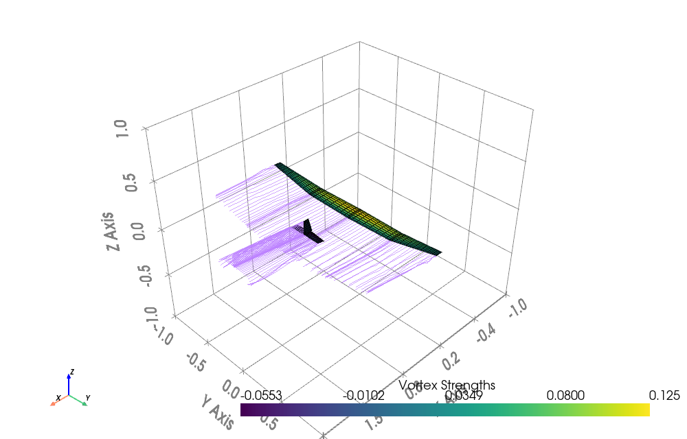
Panel density is controlled by spanwise_resolution and chordwise_resolution arguments (subdivisions per wing section), trading accuracy against cost.
7.6 Lifting-line methods
Between AeroBuildup’s empiricism and the VLM’s inviscid panels sit two lifting-line methods. Both model each wing as a line of horseshoe vortices (as in classical Prandtl theory, generalized for sweep, dihedral, and multiple surfaces), and both use NeuralFoil — the same neural-network airfoil model from Chapter 6 — for 2D viscous sectional data. That gives them something the VLM fundamentally lacks: profile drag and Reynolds-number effects, resolved section by section along the span.
For these and the validation study, we switch to a cleaner test case: a swept flying wing tested by NACA in the early 1950s (NACA RM A50K27), for which published wind-tunnel data exists.
airfoil = asb.Airfoil(
    name="n64_1_A612",
    coordinates="assets/flying-wing/n64_1_A612.dat",  # NACA 64(1)-A612 section
)

flying_wing = asb.Airplane(
    name="NACA RM A50K27 flying wing",
    xyz_ref=[0.585, 0, 0],  # Moment reference point, matching the report
    wings=[
        asb.Wing(
            name="Main Wing",
            symmetric=True,
            xsecs=[
                asb.WingXSec(xyz_le=[0, 0, 0], chord=0.4120, airfoil=airfoil),
                asb.WingXSec(xyz_le=[1.1362, 1.5490, 0], chord=0.2060, airfoil=airfoil),
            ],
        )
    ],
    c_ref=0.32,  # Reference chord used in the report
)

op_point = asb.OperatingPoint(
    atmosphere=asb.Atmosphere(altitude=0),
    velocity=91.3,  # m/s, matching the test's Reynolds number
)

print(f"Aspect ratio : {flying_wing.wings[0].aspect_ratio():.1f}")
print(f"LE sweep     : {np.arctan2d(1.1362, 1.5490):.1f} deg")
print(f"Re (c_ref)   : {op_point.reynolds(reference_length=flying_wing.c_ref):.2e}")
Aspect ratio : 10.0
LE sweep : 36.3 deg
Re (c_ref) : 2.00e+06flying_wing.draw_three_view()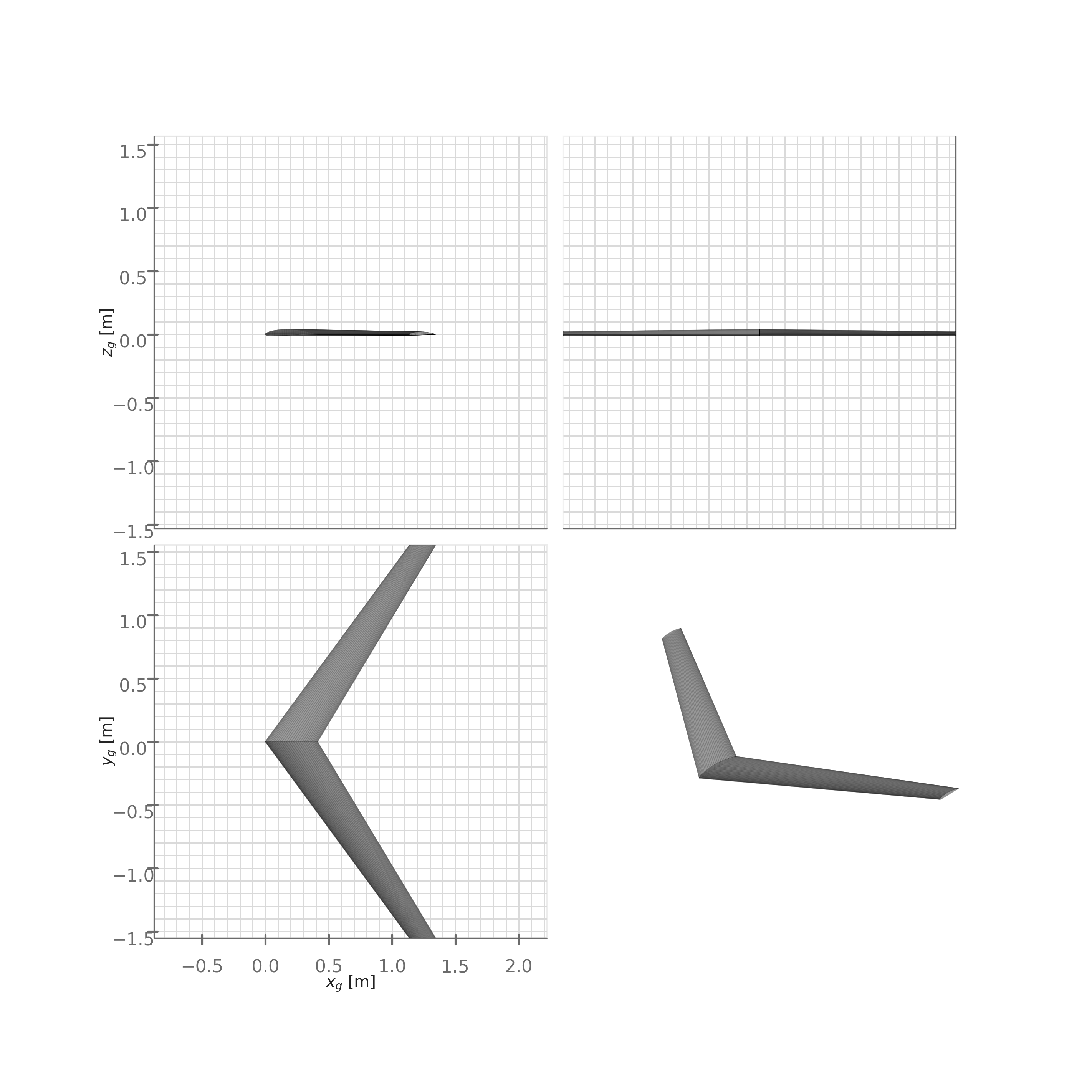
array([[<Axes3D: zlabel='$z_g$ [m]'>, <Axes3D: >],
       [<Axes3D: xlabel='$x_g$ [m]', ylabel='$y_g$ [m]'>, <Axes3D: >]],
dtype=object)<module '_common' from '/tmp/claude-1000/-home-psharpe-gh-AeroSandbox/1ccf6b40-3256-4f8d-9484-ebe00c7e55db/scratchpad/book-staging/_common.py'>7.6.1 asb.LiftingLine: quasi-linear
asb.LiftingLine solves a single linear system for the spanwise circulation (like a one-panel-chordwise VLM), then evaluates NeuralFoil at each section’s local flow condition to add viscous drag and moment. One linear solve plus one network evaluation makes it nearly VLM-cheap while still capturing viscous effects:
op = op_point.copy()
op.alpha = 5

t_start = time.time()
ll_aero = asb.LiftingLine(
    airplane=flying_wing,
    op_point=op,
).run()
t_ll = time.time() - t_start

print(f"CL = {ll_aero['CL']:.4f}, CD = {ll_aero['CD']:.4f}  ({t_ll:.2f} s)")
CL = 0.6036, CD = 0.0160 (0.09 s)Note the drag: 0.0160 includes profile drag, so it is directly comparable to wind-tunnel measurements — unlike a bare VLM number.
7.6.2 asb.NonlinearLiftingLine: implicit and stall-aware
The quasi-linear method computes circulation from linearized aerodynamics, then applies nonlinear sectional data afterward. asb.NonlinearLiftingLine closes that loop: it solves for a circulation distribution that is self-consistent with the full nonlinear NeuralFoil polars, so the lift distribution can respond to sections approaching stall. It is an ImplicitAnalysis — the governing equations become residual constraints solved by IPOPT:
t_start = time.time()
nlll_aero = asb.NonlinearLiftingLine(
    airplane=flying_wing,
    op_point=op,
    spanwise_resolution=6,  # Downsampled from the default of 8, for speed
).run()
t_nlll = time.time() - t_start

print(f"CL = {nlll_aero['CL']:.4f}, CD = {nlll_aero['CD']:.4f}  ({t_nlll:.1f} s)")
CL = 0.6115, CD = 0.0177 (7.4 s)In the linear regime it reproduces the quasi-linear answer (here, \(C_L\) within 1.3%), but each analysis costs an iterative solve — 7 s here versus 0.09 s. Reach for it when sections are working near their sectional \(C_{l,\max}\) and the lift distribution near stall is the question. If you call it standalone via .run(), it creates and solves its own asb.Opti internally; you can instead pass opti= to embed its residuals inside a larger optimization problem, so your design optimization and the aerodynamic solve converge simultaneously.
7.7 Validation: four methods vs. the wind tunnel
Talk is cheap; let’s check all four methods against the NACA wind-tunnel measurements. We sweep angle of attack with each method (AeroBuildup vectorizes; the others loop — an OperatingPoint with an array attribute is iterable, which makes the loops tidy), then overlay the published data. For context we also include results from AVL + XFoil, a classic external-tool pairing (Section 18.1).
# --- AeroBuildup: one vectorized call
ab_op = op_point.copy()
ab_op.alpha = np.linspace(-12, 14, 50)
ab_sweep = asb.AeroBuildup(airplane=flying_wing, op_point=ab_op).run()
ab_sweep["alpha"] = ab_op.alpha


def sweep(analysis_class, alphas, **kwargs):
    """Run a (non-vectorized) analysis at each alpha; stack results into arrays."""
    op_sweep = op_point.copy()
    op_sweep.alpha = alphas
    runs = [
        analysis_class(airplane=flying_wing, op_point=op_i, **kwargs).run()
        for op_i in op_sweep  # a vectorized OperatingPoint is iterable
    ]
    result = {k: np.array([r[k] for r in runs]) for k in ["CL", "CD", "Cm"]}
    result["alpha"] = alphas
    return result


vlm_sweep = sweep(asb.VortexLatticeMethod, np.linspace(-12, 14, 14),
                  spanwise_resolution=5)
ll_sweep = sweep(asb.LiftingLine, np.linspace(-12, 14, 14))
nlll_sweep = sweep(asb.NonlinearLiftingLine, np.linspace(-8, 8, 5),
                   spanwise_resolution=6)  # fewer points: each is an implicit solve
# --- Wind-tunnel data (NACA RM A50K27) and AVL+XFoil results
import pandas as pd
from scipy import interpolate
wt_CL = pd.read_excel("assets/flying-wing/NACA-RM-A50K27.xlsx", sheet_name="CL")
wt_CD = pd.read_excel("assets/flying-wing/NACA-RM-A50K27.xlsx", sheet_name="CD")
wt_Cm = pd.read_excel("assets/flying-wing/NACA-RM-A50K27.xlsx", sheet_name="CM")
# The report gives Cm vs. CL; recover alpha by interpolating the CL-vs-alpha data.
wt_Cm["alpha"] = interpolate.interp1d(
wt_CL["CL"], wt_CL["alpha"], fill_value="extrapolate"
)(wt_Cm["CL"])
avl = pd.read_csv("assets/flying-wing/avl_and_xfoil.csv") # columns: alpha, CL, CD, Cmimport _common
import matplotlib.pyplot as plt
methods = {
"AeroBuildup": (ab_sweep, _common.SERIES[0]),
"VLM (inviscid)": (vlm_sweep, _common.SERIES[1]),
"LiftingLine": (ll_sweep, _common.SERIES[2]),
"NonlinearLiftingLine": (nlll_sweep, _common.SERIES[4]),
"AVL + XFoil": (avl, _common.TEXT_SECONDARY),
}
wt_format = dict(color="black", linewidth=0, marker=".", markersize=6,
label="Wind tunnel", zorder=5)
fig, ax = plt.subplots(3, 1, figsize=(7, 11))
for name, (data, color) in methods.items():
ax[0].plot(data["alpha"], data["CL"], color=color, alpha=0.8, label=name)
ax[1].plot(data["CD"], data["CL"], color=color, alpha=0.8)
ax[2].plot(data["alpha"], data["Cm"], color=color, alpha=0.8)
ax[0].plot(wt_CL["alpha"], wt_CL["CL"], **wt_format)
ax[1].plot(wt_CD["CD"], wt_CD["CL"], **wt_format)
ax[2].plot(wt_Cm["alpha"], wt_Cm["Cm"], **wt_format)
ax[0].set_title("Lift: all methods agree while the flow stays attached")
ax[0].set_xlabel(r"Angle of attack $\alpha$ [deg]")
ax[0].set_ylabel("$C_L$ [-]")
ax[0].legend(fontsize=8, loc="lower right")
ax[1].set_title("Drag: viscous methods bracket the data; the bare VLM cannot")
ax[1].set_xlabel("$C_D$ [-]")
ax[1].set_ylabel("$C_L$ [-]")
ax[1].set_xlim(0, 1.1 * wt_CD["CD"].max())
ax[2].set_title("Moment: attached-flow methods miss the stall pitch-break")
ax[2].set_xlabel(r"Angle of attack $\alpha$ [deg]")
ax[2].set_ylabel("$C_m$ [-]")
plt.tight_layout()
plt.show()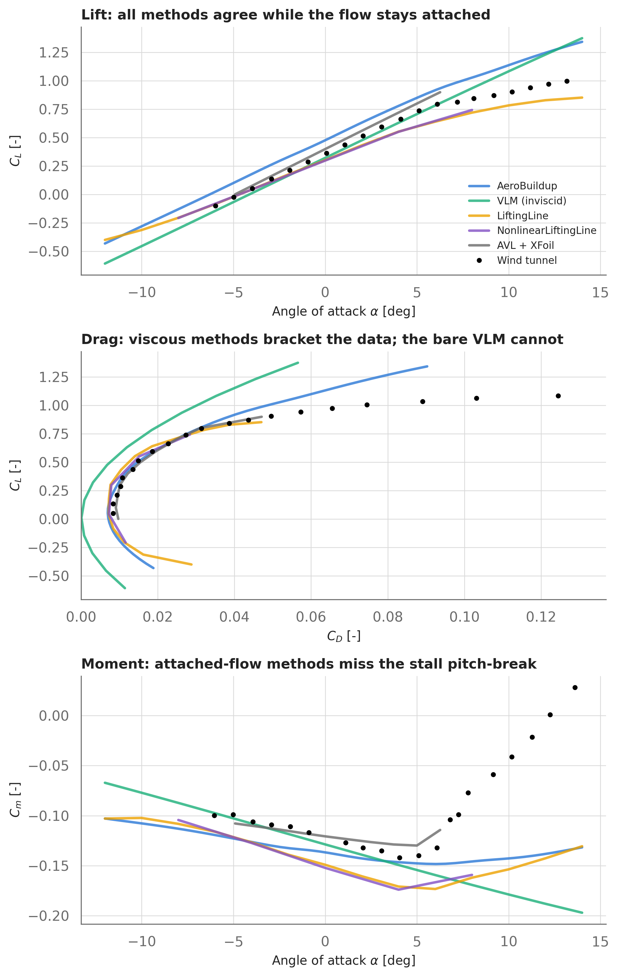
Quantitatively, the lift-curve slopes over ±4° come out as:
| Source | \(C_{L_\alpha}\) [1/rad] | vs. wind tunnel |
|---|---|---|
| Wind tunnel | 4.33 | — |
| AeroBuildup | 4.30 | -1% |
| VLM | 4.44 | +3% |
| LiftingLine | 3.65 | -16% |
| NonlinearLiftingLine | 3.64 | -16% |
What Figure 7.8 teaches about the fidelity ladder:
- In the attached-flow regime (roughly \(-6° < \alpha < 7°\)), the trends are right across the board — but accuracy differs. AeroBuildup and the VLM match the measured lift-curve slope to within a few percent; remarkably, AeroBuildup gets there without ever solving a flow equation. The lifting-line methods read about 16% low on lift-curve slope here: this planform’s 36° of sweep is exactly where a line-of-horseshoe-vortices model is weakest. Match the method to the geometry — on a high-aspect-ratio, low-sweep wing, the lifting-line methods shine.
- Drag separates the methods. The bare VLM polar hugs the \(C_D \approx C_{D_i}\) boundary — it is missing all profile drag, roughly the entire drag budget at low lift. AeroBuildup and both lifting-line methods, which include viscous sectional data, track the measured drag polar well through the drag bucket and its rise with lift.
- Stall breaks everything. Above \(\alpha \approx 7°\) the measured lift curve bends over and the measured pitching moment breaks sharply nose-up — the classic tip-stall pitch-up of swept wings, driven by separated flow that none of these attached-flow methods represent. The lesson is not “find a better fast model”; it is know your model’s envelope, and constrain your designs to stay inside it (e.g., impose a \(C_L\) margin below stall in your optimization problem).
7.8 Where to go next
- The 2D sectional models that power the lifting-line methods — NeuralFoil’s polars, their accuracy envelope, and airfoil shape optimization — are covered in Chapter 6.
- To anchor these analyses against external codes (AVL, XFoil, OpenVSP) and learn when that’s worth the friction, see Section 18.1.
- To see
VortexLatticeMethodembedded in a full design loop — coupled with structures into a wing aerostructural optimization — jump to Chapter 14.