17  Surrogate Modeling

Every model that touches an AeroSandbox optimization problem must obey one contract: it must be traceable by the automatic-differentiation machinery of Section 2.1, and smooth enough that gradients mean something. Real engineering knowledge often arrives in forms that break that contract — a spreadsheet of wind-tunnel data, a gridded atmospheric dataset, a 30-year-old Fortran code that returns one number per call. This chapter teaches the three ways AeroSandbox brings such knowledge into the differentiable world: fitting an analytical model to data (asb.FittedModel), interpolating a lookup table you can optimize through (asb.InterpolatedModel), and wrapping an unmodifiable function as a finite-differenced black box (asb.black_box). Many of AeroSandbox’s own built-in models — airfoil polars, propulsion maps, weights regressions — were produced with exactly these tools, so this chapter is also a look behind the curtain of the library itself.

17.1 Three ways to make anything differentiable

A surrogate model is a fast, smooth, differentiable stand-in for something that isn’t — data, or expensive code. The right tool depends on what you’re starting from and how much you know about the underlying physics:

Table 17.1: The surrogate-modeling toolbox, in order of preference.

Tool	You have…	You get…	Reach for it when…
asb.FittedModel	scattered data + a functional form you choose	an analytic function with optimized parameters	you know (or can guess) the shape of the physics; you want sane extrapolation and a compact, portable model
asb.InterpolatedModel	data on a structured grid	a differentiable spline lookup table, exact at the data points	the data is dense and trustworthy; you don’t want to invent a functional form
asb.UnstructuredInterpolatedModel	scattered point-cloud data	the same, after resampling onto a grid	as above, but your samples aren’t gridded
asb.black_box	a callable you can’t modify or trace	the same callable, usable in Opti, with finite-difference gradients	you can’t (or won’t) sample it offline; it’s smooth underneath; you accept slower solves

The ordering is deliberate: a fitted model is usually the best-behaved inside an optimizer, an interpolant is the fastest to build, and a black box is the honest last resort. We’ll take them in that order, using one real dataset as a through-line.

17.2 Fitting analytical models to data

17.2.1 A first fit

Start small and concrete. Imagine a temperature sensor logging a slowly-warming test rig: the true physics is linear (here, 2 °C per minute on top of a 20 °C start), each reading carries measurement noise, and at \(t = 90\) min the sensor wire comes loose and logs a bogus 0 °C. We’ll manufacture this dataset so we know the ground truth we’re trying to recover:

import aerosandbox as asb
import aerosandbox.numpy as np

np.random.seed(0)  # Reproducibility

n = 20
time = 100 * np.random.rand(n)                          # Sample times [min]
temperature = 2 * time + 20 + 10 * np.random.randn(n)   # Noisy readings [deg C]

### Add one dropout reading: the sensor wire came loose at t = 90 min.
time = np.hstack((time, 90))
temperature = np.hstack((temperature, 0))

Fitting a model to this data takes three ingredients: a model form (a function of inputs x and parameters p), the data, and an initial guess for each parameter. asb.FittedModel then finds the parameter values that make the model match the data as closely as possible:

def linear_model(x, p):
    return p["slope"] * x + p["intercept"]

fit = asb.FittedModel(
    model=linear_model,
    x_data=time,
    y_data=temperature,
    parameter_guesses={"slope": 0, "intercept": 0},
    verbose=False,  # Hides the log of the underlying optimization solve
)

print(fit.parameters)

{'slope': 1.713187613040846, 'intercept': 27.64790277922209}

There’s no magic here: under the hood, FittedModel builds an asb.Opti problem where the parameters are the design variables and the objective is the misfit — the same five-call lifecycle from Section 2.2, prepackaged. Because the optimizer is fully differentiable and second-order, this works just as well for gnarly nonlinear-in-the-parameters models as for textbook linear regression.

The result is a callable — evaluate it like a function, on scalars or arrays, on plain numbers or on optimization variables (it’s traceable, so you can drop it straight into a downstream Opti problem):

print(f"Model prediction at t = 50 min: {fit(50):.1f} deg C")
print(f"R^2 of fit:                     {fit.goodness_of_fit('R^2'):.3f}")

Model prediction at t = 50 min: 113.3 deg C
R^2 of fit:                     0.545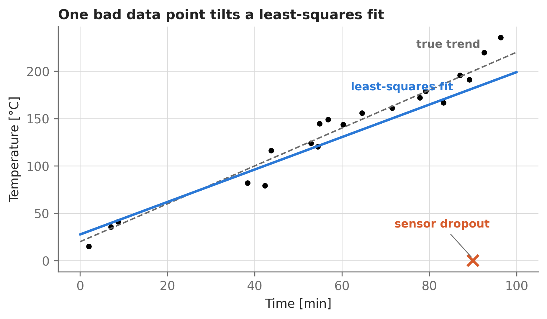

Figure 17.1: A least-squares linear fit to the sensor data. The single dropout reading drags the whole line visibly away from the true trend — one bad point out of 21 is enough.

The fit recovers a slope of 1.71 °C/min against a true value of 2 — in the right ballpark, but Figure 17.1 shows the line sagging visibly toward the dropout point. That’s a property of the default definition of “closely as possible”, which brings us to error norms.

17.2.2 Choosing the error norm

“Best fit” is not a single concept — it depends on how you penalize the residuals (the model-minus-data errors). Squaring the errors punishes large deviations harshly, so a single outlier exerts enormous leverage. Summing their absolute values treats all errors proportionally, so outliers get outvoted by the honest majority. And minimizing only the worst error hands one point total control. Let’s fit all three and look before formalizing:

def fit_with_norm(norm):
    return asb.FittedModel(
        model=linear_model,
        x_data=time,
        y_data=temperature,
        parameter_guesses={"slope": 0, "intercept": 0},
        residual_norm_type=norm,  # "L1", "L2" (default), or "Linf"
        verbose=False,
    )

fits = {norm: fit_with_norm(norm) for norm in ["L1", "L2", "Linf"]}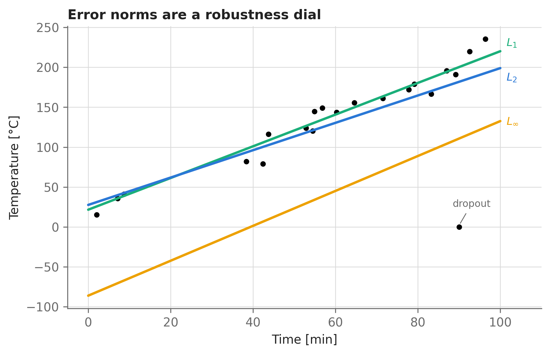

Figure 17.2: The same model, the same data, three definitions of “best”. The L1 fit shrugs off the dropout, the L2 fit tilts toward it, and the L-infinity fit is completely hijacked by it.

With the picture in mind, the definitions. Writing the residual at each data point as \(e_i = f_\text{model}(x_i) - y_i\), with per-point weights \(w_i\), the residual_norm_type argument selects which scalar gets minimized:

\[ L_1: \ \min \sum_i w_i \left| e_i \right| \qquad L_2: \ \min \sum_i w_i \, e_i^2 \qquad L_\infty: \ \min \, \max_i \left| w_i \, e_i \right| \]

The fitted slopes tell the story numerically: L1 gives 1.985 °C/min (true value: 2), L2 gives 1.713, and L∞ gives 2.186 with an intercept of -86 °C — nonsense, because the max-error criterion splits the difference with the outlier. Practical guidance:

• L2 (the default) is statistically optimal for Gaussian noise and gives the smoothest optimization landscape. Use it for clean data.
• L1 is the robust choice: outliers contribute proportionally rather than quadratically, so a few bad points barely move the fit. Use it when the data may contain glitches you haven’t scrubbed.
• L∞ minimizes the worst-case error, which is exactly what you want for a guaranteed-accuracy surrogate — but only after you’ve verified the data is outlier-free, since it is maximally outlier-sensitive.

(A nice implementation detail: absolute values and maxima are non-smooth, so FittedModel can’t just minimize them directly — internally it reformulates L1 and L∞ with slack variables and inequality constraints, the standard trick for making these norms differentiable. You get robust regression while everything stays smooth for IPOPT.)

17.2.3 Bounding fits: surrogates that never under-promise

Sometimes you don’t want the model of best fit — you want a model that’s deliberately conservative. If a surrogate feeds a drag estimate into a sizing loop, a fit that’s wrong by +5% in the optimizer’s favor produces an airplane that misses spec; a fit guaranteed to sit at-or-above the data can’t be gamed that way. The fit_type argument adds a one-sided constraint to the internal fitting problem, forcing the model to stay on one side of every data point (we’ll drop the dropout reading first — bounding fits are, by construction, even more outlier-sensitive than L∞):

time_clean = time[:-1]  # Drop the dropout point
temperature_clean = temperature[:-1]

def fit_with_type(fit_type):
    return asb.FittedModel(
        model=linear_model,
        x_data=time_clean,
        y_data=temperature_clean,
        parameter_guesses={"slope": 0, "intercept": 0},
        fit_type=fit_type,  # "best" (default), "upper bound", or "lower bound"
        residual_norm_type="L1",  # L1 pairs well with bounding fits
        verbose=False,
    )

bound_fits = {ft: fit_with_type(ft) for ft in ["best", "upper bound", "lower bound"]}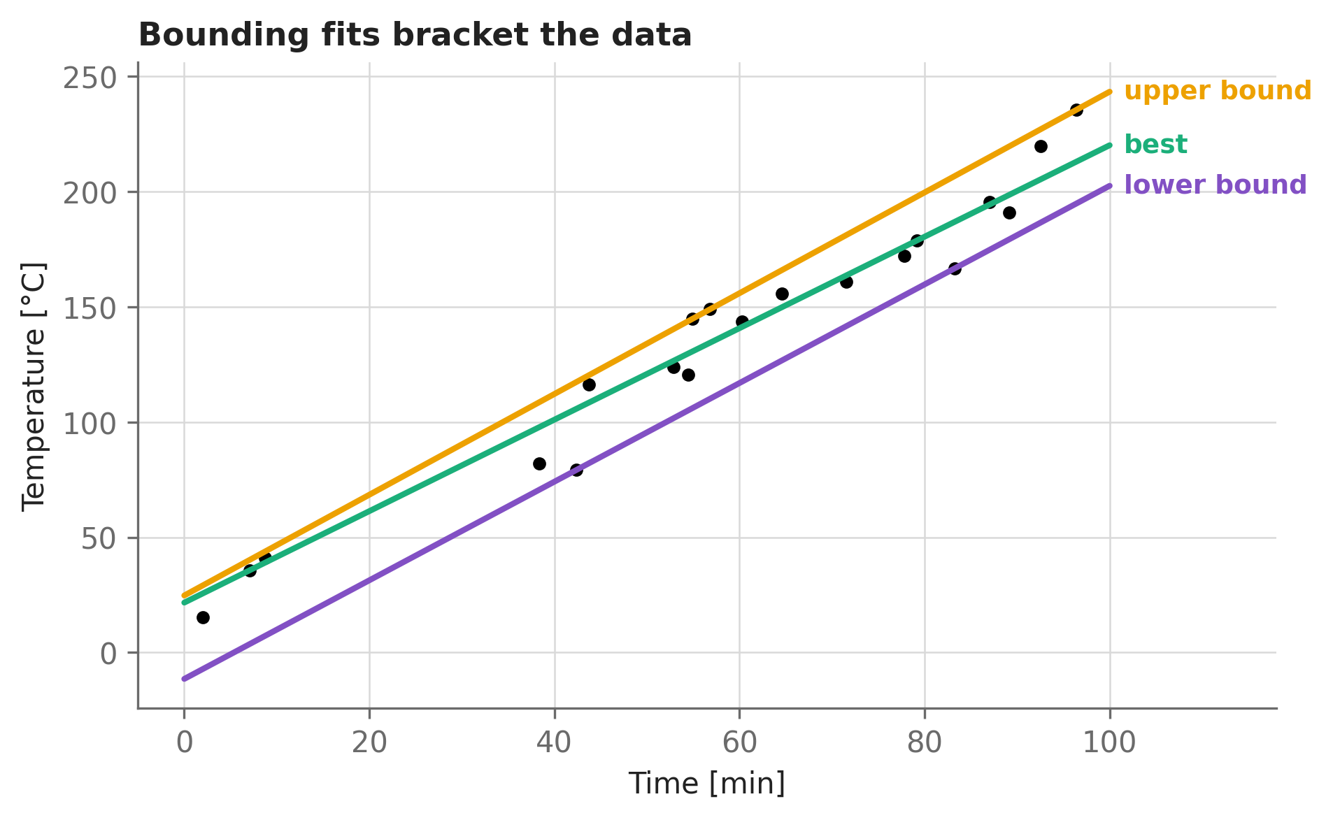

Figure 17.3: Best-fit, upper-bound, and lower-bound fits to the cleaned sensor data. The bounding fits touch the extreme data points but never cross them — a conservative envelope for robust design.

Fitting both an upper- and lower-bound model gives you an envelope on the quantity being modeled — useful for propagating “the data could be anywhere in here” through a design study without full-blown uncertainty quantification.

TipPercent error instead of absolute error

One more knob worth knowing: put_residuals_in_logspace=True minimizes the error of \(\ln(f_\text{model})\) against \(\ln(y)\), i.e. percent error rather than absolute error. This is the right choice for quantities spanning orders of magnitude (Reynolds number effects, mass regressions across UAVs-to-airliners), where an absolute-error fit would ignore the small end of the dataset entirely. It requires all data and model outputs to be positive.

17.2.4 A real fit: continental-U.S. wind speeds

Now the real thing. High-altitude long-endurance (HALE) aircraft must penetrate winds to stationkeep, so a key design input is: how strong are the worst winds, as a function of latitude and altitude? The AeroSandbox repository ships a dataset of 99th-percentile wind speeds over the continental U.S. (August conditions, 1979–2020, derived from reanalysis data) on a latitude–altitude grid — real data, with real structure: calm near the surface, a violent jet-stream ridge near 10–12 km, and a quiet lull in the lower stratosphere.

from pathlib import Path
from scipy import io

data_file = (
    Path(asb.__file__).parent.parent
    / "tutorial" / "05 - Surrogate Modeling" / "01 - Fitting"
    / "data" / "wind_data_99.mat"
)
if not data_file.exists():  # e.g. pip-installed AeroSandbox, without the repo
    import urllib.request
    data_file, _ = urllib.request.urlretrieve(
        "https://github.com/peterdsharpe/AeroSandbox/raw/master/tutorial/"
        "05%20-%20Surrogate%20Modeling/01%20-%20Fitting/data/wind_data_99.mat",
        "wind_data_99.mat",
    )

data = io.loadmat(str(data_file))
latitudes = data["lats"].flatten().astype(float)[::-1]     # [deg N], ascending
altitudes = data["alts"].flatten()[::-1]                   # [m], ascending
speeds_grid = (                                            # [m/s], shape (93, 37)
    data["speeds"].reshape(len(altitudes), len(latitudes)).T[::-1, ::-1]
)

### Also make flattened (unstructured) versions, which is what fitting wants:
Lats, Alts = np.meshgrid(latitudes, altitudes, indexing="ij")
lats_flat = Lats.flatten()
alts_flat = Alts.flatten()
speeds_flat = speeds_grid.flatten()

print(f"{len(latitudes)} latitudes x {len(altitudes)} altitudes = {len(speeds_flat)} data points")

93 latitudes x 37 altitudes = 3441 data points

Two pieces of preprocessing make the difference between a fit that converges crisply and one that fights you. First, scale everything to order-one: the raw inputs span 26–49°N and 100–48,500 m — three orders of magnitude apart — and Section 3.4 taught us what badly-scaled variables do to a solver. Second, weight the data points sensibly: this grid is much denser at low altitude, so an unweighted fit would obsess over the boundary layer; weighting each point by the altitude interval it represents (a trapezoidal weighting) restores balance.

### Scale inputs and output to roughly [-1, 1]
lats_scaled = (lats_flat - 37.5) / 11.5
alts_scaled = (alts_flat - 24200) / 24200
speeds_scaled = (speeds_flat - 7) / 56

### Weight each point by the altitude interval it represents
alt_spacing = np.diff(altitudes)
alt_spacing = np.hstack((alt_spacing[0], alt_spacing, alt_spacing[-1]))
weights_1D = (alt_spacing[:-1] + alt_spacing[1:]) / 2
weights = np.tile(weights_1D / np.mean(weights_1D), (len(latitudes), 1)).flatten()

Choosing the model form is the creative step in any fit, and it’s physics-informed curve sculpting: we superpose a quadratic bowl in each variable (the large-scale trend), a generalized-Gaussian bump (the jet stream), and low-order cross terms (the jet’s tilt with latitude). That’s 18 parameters for 3,441 data points. Note the parameter_bounds argument — bounds keep the fit inside the regime where the model form is well-posed (spreads must be positive; exponents near 2 keep the bump bump-shaped):

def wind_model(x, p):
    lat = x["latitude_scaled"]
    alt = x["altitude_scaled"]
    return (
        p["c0"]                                       # Constant
        + p["cql"] * (lat - p["lqc"]) ** 2            # Quadratic in latitude
        + p["cqa"] * (alt - p["aqc"]) ** 2            # Quadratic in altitude
        + p["cqla"] * lat * alt                       # Quadratic cross-term
        + p["cg"] * np.exp(                           # Jet-stream bump:
            -(
                np.fabs(lat - p["lgc"]) ** p["lgh"] / (2 * p["lgs"] ** 2)
                + np.fabs(alt - p["agc"]) ** p["agh"] / (2 * p["ags"] ** 2)
                + p["cgc"] * lat * alt
            )
        )
        + p["c4a"] * (alt - p["c4c"]) ** 4            # Quartic in altitude
        + p["c12"] * lat * alt**2                     # Cubic cross-terms
        + p["c21"] * lat**2 * alt
    )

wind_fit = asb.FittedModel(
    model=wind_model,
    x_data={  # Multiple inputs: pass a dict of arrays...
        "latitude_scaled": lats_scaled,
        "altitude_scaled": alts_scaled,
    },
    y_data=speeds_scaled,
    parameter_guesses={
        "c0": -0.5, "cql": 0.02, "lqc": 4, "cqa": 0.2, "aqc": -1.5, "cqla": -0.1,
        "cg": 0.8, "lgc": 0.7, "lgh": 2, "lgs": 1, "agc": -0.5, "agh": 2,
        "ags": 0.15, "cgc": 0.3, "c4a": 0.02, "c4c": 1, "c12": 0.08, "c21": -0.03,
    },
    parameter_bounds={  # Keep the model form well-posed:
        "lgs": (0, None), "ags": (0, None),  # Gaussian spreads must be positive
        "lgh": (1, 3), "agh": (1, 3),        # Exponents near 2 keep the bump bump-shaped
    },
    weights=weights,
    verbose=False,
)

print(f"R^2 = {wind_fit.goodness_of_fit('R^2'):.4f}")
print(f"RMS error = {wind_fit.goodness_of_fit('rms') * 56:.2f} m/s")

R^2 = 0.9600
RMS error = 2.63 m/s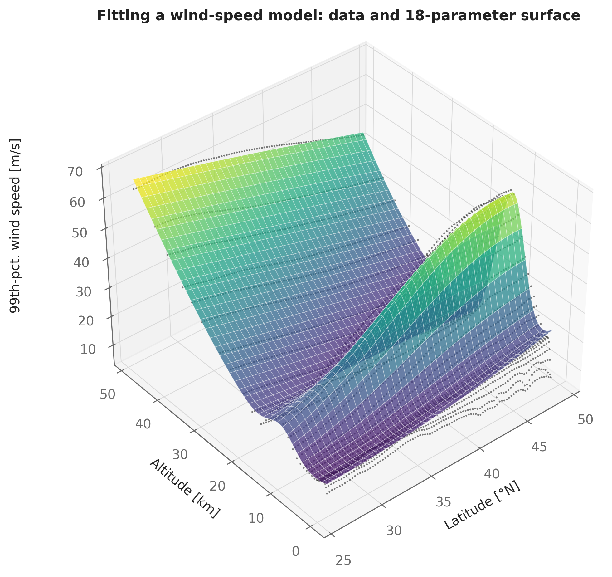

Figure 17.4: An 18-parameter analytical fit (surface) to 3,441 measured 99th-percentile wind speeds (dots). The ridge near 10–12 km altitude is the jet stream; the trough above it, near 20 km, is the stratospheric lull that HALE aircraft loiter in.

The result: R² of 0.960 and an RMS error of 2.6 m/s across the whole domain — from 18 numbers you could print on a business card. This compactness is the deep advantage of fitting over interpolation: the surrogate is portable (no dataset to ship), it smooths measurement noise instead of reproducing it, and because the functional form encodes physics, it extrapolates like physics instead of like a polynomial having a bad day. The price is that you must choose that form, and the fit is only as good as your choice — always check goodness_of_fit() and, more importantly, plot the residuals before trusting one.

17.3 Lookup tables you can optimize through

17.3.1 Interpolation in one dimension

Sometimes there’s no obvious functional form, or you simply trust the data more than any curve you’d sculpt through it. Then you want a lookup table — but an ordinary table lookup is piecewise-something, and “piecewise” is exactly what gradient-based optimizers hate. asb.InterpolatedModel solves this by building a B-spline interpolant: it passes exactly through your data points, is twice-differentiable everywhere, and is traceable by the AD system, so the optimizer can march right through it.

Concretely: suppose flight testing of a small electric UAV produced a table of electrical power required versus airspeed at nine test points. (We’ll manufacture the “flight-test data” from a textbook power model — profile drag growing as \(V^3\), induced drag shrinking as \(1/V\) — so that we have an exact truth to grade the interpolant against.)

rho = 1.225   # Air density [kg/m^3]
W = 50.0      # Aircraft weight [N]
S = 0.5       # Wing area [m^2]
CD0 = 0.03    # Zero-lift drag coefficient [-]
k = 1 / (np.pi * 0.9 * 12)  # Induced drag factor, e = 0.9, AR = 12 [-]

def power_true(V):  # The "true physics" the table secretly comes from
    q = 0.5 * rho * V**2                # Dynamic pressure [Pa]
    CL = W / (q * S)                    # Lift coefficient in level flight [-]
    return q * S * (CD0 + k * CL**2) * V  # Power = drag * speed [W]

V_table = np.linspace(6, 30, 9)   # Flight-test airspeeds [m/s]
P_table = power_true(V_table)     # Measured power [W]

power_spline = asb.InterpolatedModel(V_table, P_table)                   # method="bspline"
power_linear = asb.InterpolatedModel(V_table, P_table, method="linear")  # for comparison

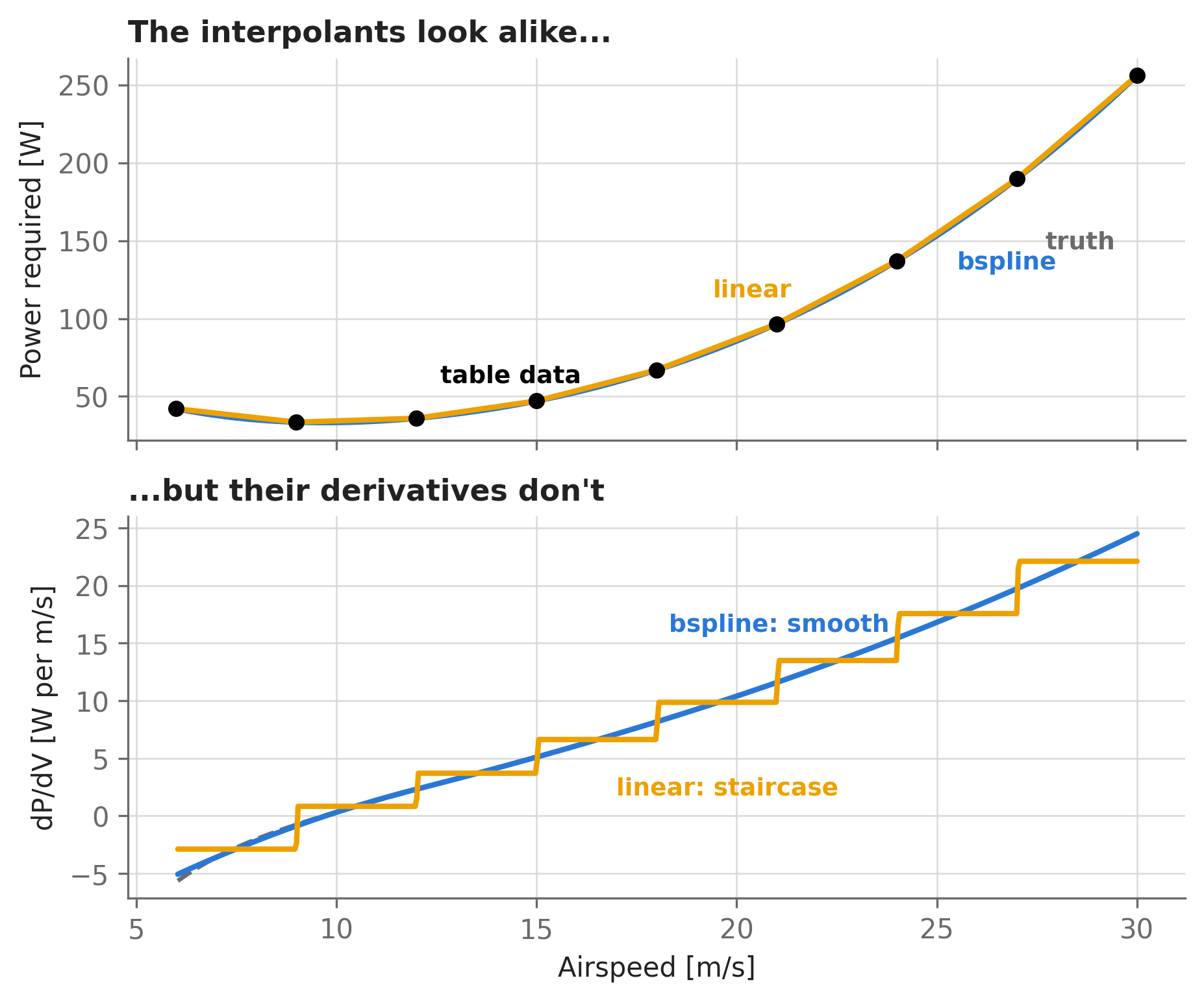
Why insist on the spline? Look not just at the interpolant but at its derivative — the thing the optimizer actually consumes:

Figure 17.5: Top: both interpolation methods look reasonable at a glance. Bottom: their derivatives — what the optimizer actually sees — differ completely. The linear table’s staircase derivative gives Newton’s method nothing to work with; the spline’s smooth derivative behaves like real physics.

Now the payoff: optimize through the table. Minimum power required means maximum endurance, so let’s ask the spline for the best loiter speed. One critical habit: by default an InterpolatedModel returns NaN outside its data range (extrapolating a spline is asking for fiction), and NaNs kill solves — so always bound any variable that feeds a lookup table to the table’s domain:

opti = asb.Opti()

V = opti.variable(
    init_guess=15,
    lower_bound=V_table.min(),  # Never let the optimizer leave the table!
    upper_bound=V_table.max(),
)
opti.minimize(power_spline(V))

sol = opti.solve(verbose=False)

V_best_table = sol(V)
V_best_true = (W / (0.5 * rho * S) * np.sqrt(k / (3 * CD0))) ** 0.5  # Analytic optimum
print(f"Best-endurance speed, from 9-point table: {V_best_table:.3f} m/s")
print(f"Best-endurance speed, analytic truth:     {V_best_true:.3f} m/s")

Best-endurance speed, from 9-point table: 9.710 m/s
Best-endurance speed, analytic truth:     9.666 m/s

A nine-point table locates the optimum within 0.044 m/s of the truth. And the error is controlled by the only knob a lookup table has — resolution:

for n_points in [9, 17, 33]:
    V_t = np.linspace(6, 30, n_points)
    table = asb.InterpolatedModel(V_t, power_true(V_t))

    opti = asb.Opti()
    V = opti.variable(init_guess=15, lower_bound=6, upper_bound=30)
    opti.minimize(table(V))
    sol = opti.solve(verbose=False)

    print(f"{n_points:3} points -> V* = {sol(V):.4f} m/s "
          f"(error: {abs(sol(V) - V_best_true):.1e} m/s)")

  9 points -> V* = 9.7096 m/s (error: 4.4e-02 m/s)
 17 points -> V* = 9.6678 m/s (error: 1.8e-03 m/s)
 33 points -> V* = 9.6658 m/s (error: 1.6e-04 m/s)

Each doubling of table resolution cuts the argmin error by more than an order of magnitude — smooth-function spline convergence working in your favor. Two caveats to keep in mind, both inherited from cubic splines generally: they can overshoot between points of rapidly-varying data (Runge’s phenomenon — if your data is noisy, smooth or fit it instead of interpolating it, since an interpolant faithfully reproduces every wiggle of noise), and method="linear" — kinked but monotonicity-preserving — is better reserved for plotting and sanity checks than for optimization, as Figure 17.5 showed.

17.3.2 N-dimensional tables and vectorized solves

The same class scales to N dimensions when your data lives on a structured grid — you supply the grid axes as a dict of 1D coordinate arrays and the values as an N-dimensional array. The wind dataset from Section 17.2.4 is exactly that shape, so this time, instead of sculpting an 18-parameter function, we just wrap the grid directly:

wind_table = asb.InterpolatedModel(
    x_data_coordinates={
        "latitude": latitudes,   # (93,) [deg N] -- must be strictly increasing
        "altitude": altitudes,   # (37,) [m]     -- must be strictly increasing
    },
    y_data_structured=speeds_grid,  # (93, 37) [m/s]
)

print(f"Wind at 35 deg N, 20 km: {wind_table({'latitude': 35, 'altitude': 20e3}):.1f} m/s")

Wind at 35 deg N, 20 km: 14.9 m/s

WarningGrid coordinates must be strictly increasing

Meteorological and CFD datasets frequently store axes in descending order (this one does — pressure levels, top-down). InterpolatedModel requires strictly increasing coordinates and will refuse otherwise; that’s why the loading cell earlier flipped both axes ([::-1]) and the data grid to match. Getting an axis flip wrong scrambles the table silently, so spot-check a few values (as above) against the raw data after building any table.

Calls broadcast over arrays — including arrays of optimization variables, which enables a wonderfully compact pattern: solving many design problems in a single Opti. The design question from earlier — where is the stratospheric wind lull? — is really 93 questions, one per latitude. Rather than looping, declare a vector of 93 altitude variables and minimize the sum of wind speeds; since each altitude affects only its own latitude’s wind speed, the problems are independent and IPOPT solves them simultaneously:

opti = asb.Opti()

loiter_altitude = opti.variable(
    init_guess=20e3 * np.ones(len(latitudes)),  # One variable per latitude [m]
    lower_bound=15e3,   # Stay above weather and traffic...
    upper_bound=45e3,   # ...and inside the table domain.
)
wind_at_loiter = wind_table({
    "latitude": latitudes,        # Fixed data...
    "altitude": loiter_altitude,  # ...paired with optimization variables.
})

opti.minimize(np.sum(wind_at_loiter))

sol = opti.solve(verbose=False)
best_altitude = sol(loiter_altitude)
best_wind = sol(wind_at_loiter)

print(f"Optimal loiter altitudes span {best_altitude.min() / 1e3:.1f} "
      f"to {best_altitude.max() / 1e3:.1f} km")
print(f"Worst-case wind at those altitudes: {best_wind.max():.1f} m/s")

Optimal loiter altitudes span 17.0 to 21.0 km
Worst-case wind at those altitudes: 16.4 m/s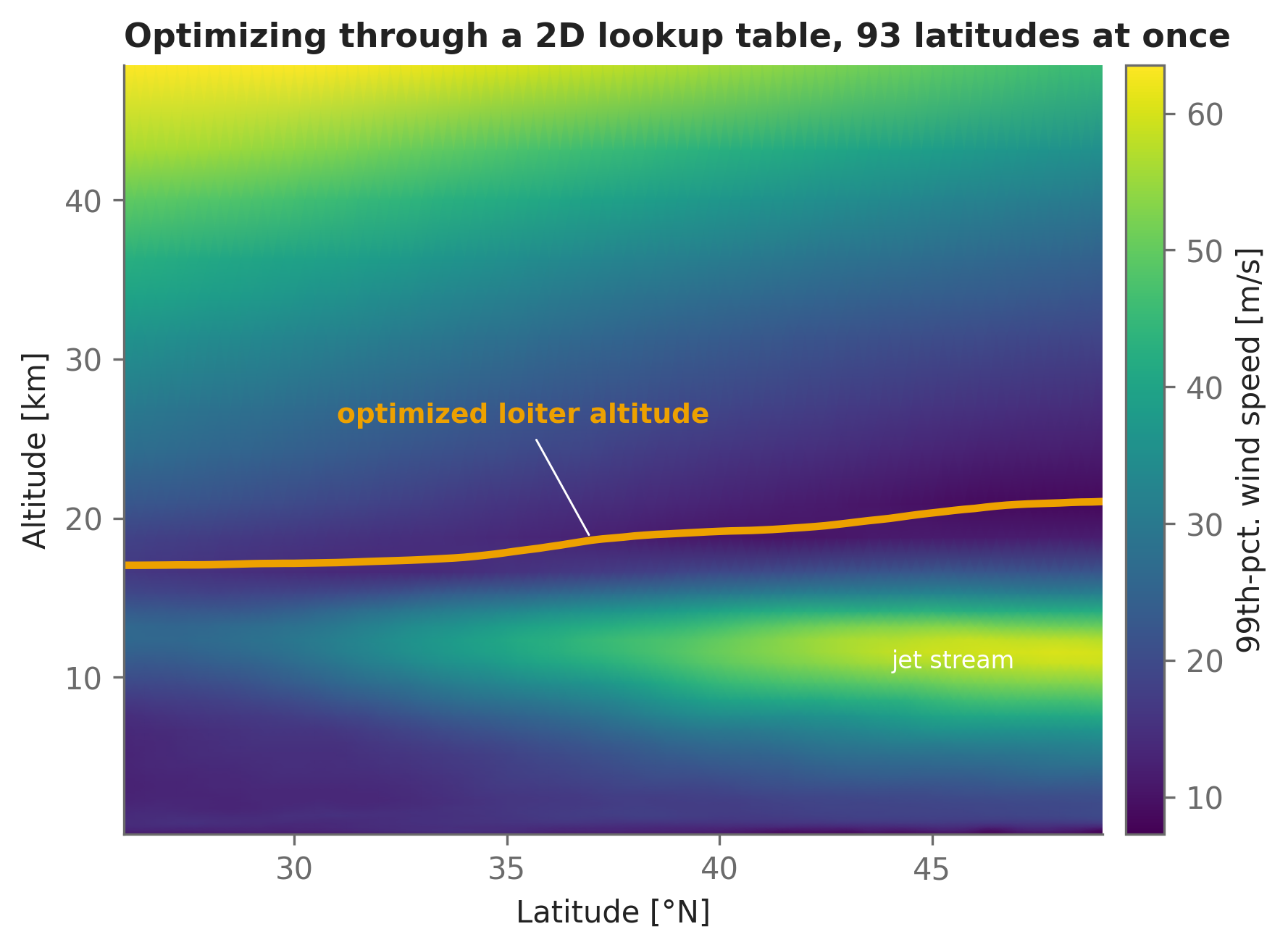

Figure 17.6: The 99th-percentile wind field (color), with the optimized minimum-wind loiter altitude at each latitude (line). The optimizer traces the stratospheric lull above the jet stream — the quiet corridor where solar HALE aircraft fly.

One Opti, 93 variables, one solve, a fraction of a second — and a designer’s answer: over the continental U.S., the August wind lull sits near 19 km, with 99th-percentile winds as low as 8 m/s at southern latitudes. This “vector of independent sub-problems” trick reappears throughout the book, from airfoil polars to trajectory collocation.

17.3.3 Unstructured data: point clouds

If your samples don’t lie on a grid — scattered CFD runs, flight-test points, a Latin-hypercube DOE — asb.UnstructuredInterpolatedModel bridges the gap: it first fits a radial-basis-function interpolator through the point cloud, uses it to resample onto a structured grid, then proceeds exactly as above (so the model you optimize through is still a well-behaved B-spline). Here it is reconstructing the wind field from 500 random samples of it:

np.random.seed(0)
n_samples = 500
lat_scatter = np.random.uniform(26, 49, n_samples)
alt_scatter = np.random.uniform(200, 48e3, n_samples)
wind_scatter = wind_table({"latitude": lat_scatter, "altitude": alt_scatter})

wind_from_scatter = asb.UnstructuredInterpolatedModel(
    x_data={"latitude": lat_scatter, "altitude": alt_scatter},
    y_data=wind_scatter,
    x_data_resample=40,  # Resample the point cloud onto a 40 x 40 grid
)

query = {"latitude": 35, "altitude": 20e3}
print(f"Reconstructed from 500 scattered points: {wind_from_scatter(query):.1f} m/s")
print(f"Full 3,441-point gridded table:          {wind_table(query):.1f} m/s")

Reconstructed from 500 scattered points: 16.3 m/s
Full 3,441-point gridded table:          14.9 m/s

The reconstruction is decent but not exact — RBF resampling is a smoother, not an oracle, and its quality degrades quickly in sparsely-sampled corners of the domain. For scattered data of modest size, also weigh the alternative: an asb.FittedModel with a physics-informed form (as in Section 17.2.4) often extracts more truth from fewer scattered points than any generic interpolant can.

17.4 Wrapping black-box functions

Sometimes you can’t get the data out in advance: the model is a piece of code — a vendor’s compiled library, a legacy script, a numerical simulation — that you can call but not trace. Suppose our wind model lived inside exactly such a function (here we’ll build one from SciPy, which AD cannot see through — note it demands and returns plain floats, like real legacy code):

from scipy.interpolate import RegularGridInterpolator

_legacy_interp = RegularGridInterpolator(
    (latitudes, altitudes), np.array(speeds_grid), method="cubic",
)

def wind_speed_legacy(latitude, altitude):
    """Pretend this is 30-year-old code you cannot modify or differentiate."""
    return float(_legacy_interp([float(latitude), float(altitude)])[0])

Feed an optimization variable into this function and it fails immediately — a symbolic variable is not a number, so float() has nothing to convert (this is the same reason plain numpy functions can’t be used on Opti variables, per Section 2.5):

opti = asb.Opti()
altitude = opti.variable(init_guess=20e3)

try:
    opti.minimize(wind_speed_legacy(35.0, altitude))
except Exception as e:
    print(f"{type(e).__name__}: {str(e)[:60]}...")

RuntimeError: .../casadi/core/mx_node.cpp:477: 'to_double' not defined for...

asb.black_box makes such a function usable anyway. It wraps the callable so that, whenever the solver needs a derivative, the wrapper computes one by finite differences — automatically, behind the scenes:

import time as timer

wind_speed_bb = asb.black_box(
    function=wind_speed_legacy,
    fd_method="central",  # or "forward", "backward", "smoothed"
)

t_start = timer.perf_counter()

opti = asb.Opti()
altitude = opti.variable(init_guess=20e3, lower_bound=15e3, upper_bound=45e3)
opti.minimize(wind_speed_bb(35.0, altitude))  # Positional or keyword args both work
sol_bb = opti.solve(verbose=False)

t_blackbox = timer.perf_counter() - t_start
iters_blackbox = sol_bb.stats()["iter_count"]
altitude_blackbox = sol_bb(altitude)

print(f"Minimum-wind altitude: {altitude_blackbox / 1e3:.2f} km "
      f"({iters_blackbox} iterations, {t_blackbox * 1e3:.0f} ms)")

Minimum-wind altitude: 17.84 km (17 iterations, 123 ms)

It works — and it agrees with the native, fully-traced lookup table from the previous section. But compare the cost of the same solve done natively:

t_start = timer.perf_counter()

opti = asb.Opti()
altitude = opti.variable(init_guess=20e3, lower_bound=15e3, upper_bound=45e3)
opti.minimize(wind_table({"latitude": 35.0, "altitude": altitude}))
sol_native = opti.solve(verbose=False)

t_native = timer.perf_counter() - t_start
iters_native = sol_native.stats()["iter_count"]
altitude_native = sol_native(altitude)

print(f"Minimum-wind altitude: {altitude_native / 1e3:.2f} km "
      f"({iters_native} iterations, {t_native * 1e3:.0f} ms)")

Minimum-wind altitude: 17.84 km (5 iterations, 66 ms)

Same answer (to within 0.1 m), but the black-box route took 17 iterations versus 5 — the optimizer is flying on noisy, approximate derivatives instead of exact ones, and it shows. On this toy problem both finish quickly; on a problem with hundreds of variables, the gap becomes decisive.

WarningBlack boxes: the honest fine print

asb.black_box is a pragmatic escape hatch, not a free lunch. Know what you’re signing up for:

• Gradient cost scales with input count. Central differencing costs about \(2n\) extra function evaluations per gradient of an \(n\)-input function — per constraint or objective, per iteration. Exact-AD gradients via aerosandbox.numpy cost roughly one extra evaluation, regardless of \(n\).
• Finite differences amplify noise. If the function has any internal noise (iterative solvers with loose tolerances, mesh regeneration, file round-trips), differencing turns small output jitter into large gradient garbage — typically visible as IPOPT grinding without converging. The function must be smooth underneath, even though you can’t see inside it.
• No exact second derivatives — expect more iterations, as above.
• Scalar-in, scalar-out. Each argument must be a scalar, and (currently) only single-output functions are supported. Vectorization is lost: every evaluation is a round-trip through the Python callback.
• Every call at solve time is a real call. If the wrapped function takes minutes (CFD, FEA), the optimizer’s thousands of evaluations are minutes each. In that regime, don’t optimize through the tool — sample it offline (tens-to-hundreds of runs, embarrassingly parallel), then build a FittedModel or InterpolatedModel from the results and optimize through that instead. That workflow — external tools generating data for surrogates — is the subject of Section 18.1.

17.5 Choosing your surrogate: a field guide

Collecting the chapter into four rules of thumb:

1. Know the shape of the physics? Fit it (FittedModel). You get compactness, noise rejection, and physically-sane extrapolation. Scale your inputs, pick the norm to match your outlier situation, and bound parameters to keep the form well-posed.
2. Dense, trusted, gridded data? Interpolate it (InterpolatedModel, default B-spline). Exact at the data, C²-smooth for the optimizer — just bound your variables to the table domain, and never interpolate noise you’d rather smooth.
3. Scattered data, no model form in mind? UnstructuredInterpolatedModel — or reconsider option 1.
4. Untouchable code? black_box if it’s smooth, fast, and low-dimensional; otherwise sample offline and go to options 1–2.

17.6 Where to go next

• Section 6.1 shows this chapter’s philosophy at industrial strength: NeuralFoil, a neural-network surrogate trained on tens of millions of viscous airfoil analyses, giving XFoil-class answers at optimization-friendly speed and smoothness.
• Section 18.1 covers the other half of the black-box story — running external codes like XFoil and AVL from AeroSandbox, and harvesting their outputs as training data for the surrogates you now know how to build.
• Chapter 3 is worth rereading with surrogate eyes: the scaling, smoothness, and NaN-safety lessons there are precisely what make a fitted or interpolated model behave inside a large design problem.