This chapter shows how to solve differential equations — and then optimize through them — using the same asb.Opti interface you already know from design problems. You’ll learn the simultaneous (“direct collocation”) approach that AeroSandbox uses for dynamics: instead of marching an ODE forward in time, you pose the entire time history as optimization variables and let the solver find all of it at once. We build up from a classic boundary-layer ODE (where this approach makes hard inverse problems trivial), to a minimum-effort control problem, to a free-final-time problem where bang-bang control emerges on its own — and we finish with the convergence check you should run on every trajectory problem before you trust it. This machinery is the foundation for the aircraft dynamics stack in Section 13.1 and the coupled aerostructural study in Chapter 14.
12.1 An ODE is just a set of constraints
AeroSandbox has no ODE integrator in the scipy.integrate.solve_ivp sense — and that is a feature. A time-marching integrator computes the state at step \(i+1\) from the state at step \(i\), which means it can only answer one narrow question: “given complete initial conditions, what happens next?” Most engineering questions aren’t shaped like that. Boundary-value problems pin down conditions at both ends. Optimal control asks for the input history that extremizes something. Design optimization wants the wing area and the trajectory it flies, together.
The simultaneous approach handles all of these with one idea: treat the sampled time history of every state as a vector of optimization variables, and treat the ODE itself as a set of equality constraints tying those samples together. The solver then finds the whole trajectory at once, in the same Newton iteration that handles your boundary conditions, path constraints, and objective. In the trajectory-optimization literature this is called direct collocation; Matthew Kelly’s tutorial paper An Introduction to Trajectory Optimization is an excellent companion reference for this chapter.
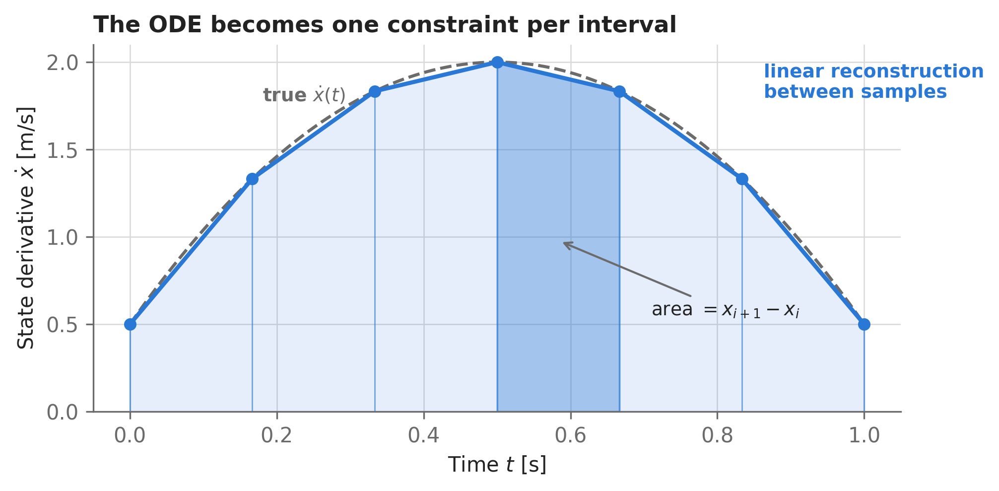
Concretely: to represent an unknown function \(x(t)\), we sample it at \(N\) points \(t_1 < t_2 < \dots < t_N\) and track the values \(x_i = x(t_i)\) as optimization variables. Between samples, we assume the derivative\(\dot{x}(t)\) varies linearly — so the state change across each interval is the area of a trapezoid:
Figure 12.1: Trapezoidal collocation. The unknown derivative \(\dot{x}(t)\) (dashed gray) is tracked only at discrete samples (dots); a linear reconstruction (blue) fills in between. Each shaded trapezoid’s area must equal the change in the state \(x\) across that interval — and each such requirement becomes one equality constraint in the optimization problem.
In symbols: given a first-order ODE \(\dot{x} = f(x, u, t)\) with sampled states \(x_i\) and sampled derivatives \(f_i = f(x_i, u_i, t_i)\), trapezoidal collocation imposes
That’s \(N-1\) equality constraints per state — large but extremely sparse, which is exactly the structure IPOPT is built to exploit. Higher-order ODEs pose no difficulty: any \(n\)-th-order ODE decomposes into \(n\) first-order ODEs by introducing the intermediate derivatives as states (we’ll do this to a third-order ODE in a moment).
AeroSandbox wraps this pattern in two Opti methods:
opti.derivative_of(variable, with_respect_to, derivative_init_guess) — creates a new variable defined to be the derivative of an existing one, and adds the collocation constraints tying them together. Use it to build chains like position → velocity → acceleration.
opti.constrain_derivative(derivative, variable, with_respect_to) — constrains an existing expression to be the derivative of an existing variable. Use it to “close the loop” with your physics, e.g. \(\mathrm{d}v/\mathrm{d}t = F/m\).
Both accept a method= argument ("trapezoidal" by default; also "forward_euler", "backward_euler", "simpson", "cubic", and others — see asb.numpy.integrate_discrete_intervals() for the full list). Note that all methods are expressed as integrators rather than differentiators, which keeps the constraints well-conditioned as the timestep shrinks.
12.2 Solving a hard ODE: the Falkner–Skan boundary layer
Before adding any objective, let’s use this machinery as a pure ODE solver — on a problem where time-marching genuinely struggles. The Falkner–Skan equation describes the self-similar laminar boundary layer on a wedge, where the edge velocity varies as \(u_e \propto x^a\). The exponent \(a\) encodes the pressure gradient: \(a = 0\) is a flat plate (the Blasius solution), \(a > 0\) is a favorable (accelerating) gradient like a wing’s leading edge, and \(a < 0\) is an adverse gradient that pushes the boundary layer toward separation.
Written as a system of first-order ODEs in the similarity coordinate \(\eta\) (following Drela’s Aerodynamics of Viscous Fluids notation, with \(F\) the normalized streamfunction, \(U\) the velocity profile, and \(S\) the shear profile):
\[
F' = U, \qquad
U' = S, \qquad
S' = -\frac{1+a}{2} F S - a \left(1 - U^2\right),
\]
This is a good stress test: it’s nonlinear, it’s third-order, and it’s a two-point boundary-value problem — conditions are pinned at both walls of the domain, so explicit forward integration would require shooting, which is notoriously unstable for this equation. With collocation, none of that matters. We declare \(F\) as a variable, chain \(U\) and \(S\) off it with derivative_of(), and close the loop with constrain_derivative():
import aerosandbox as asbimport aerosandbox.numpy as npopti = asb.Opti()a = opti.parameter(value=0.1) # Pressure-gradient exponent: u_e ~ x^an_points =100eta = np.linspace(0, 10, n_points) # Discretized similarity coordinateF = opti.variable( # Normalized streamfunction F(eta) init_guess=eta +10/3* (1- eta /10) **3, # integral of the guess for U)U = opti.derivative_of( # Velocity profile U(eta) = F' F, with_respect_to=eta, derivative_init_guess=1- (1- eta /10) **2, # guess a quadratic profile)S = opti.derivative_of( # Shear profile S(eta) = U' U, with_respect_to=eta, derivative_init_guess=0.2* (1- eta /10), # derivative of the guess for U)opti.constrain_derivative( # The governing equation: S' = ... variable=S, with_respect_to=eta, derivative=-(1+ a) /2* F * S - a * (1- U**2),)opti.subject_to([ F[0] ==0, U[0] ==0, U[-1] ==1,])sol = opti.solve(verbose=False)
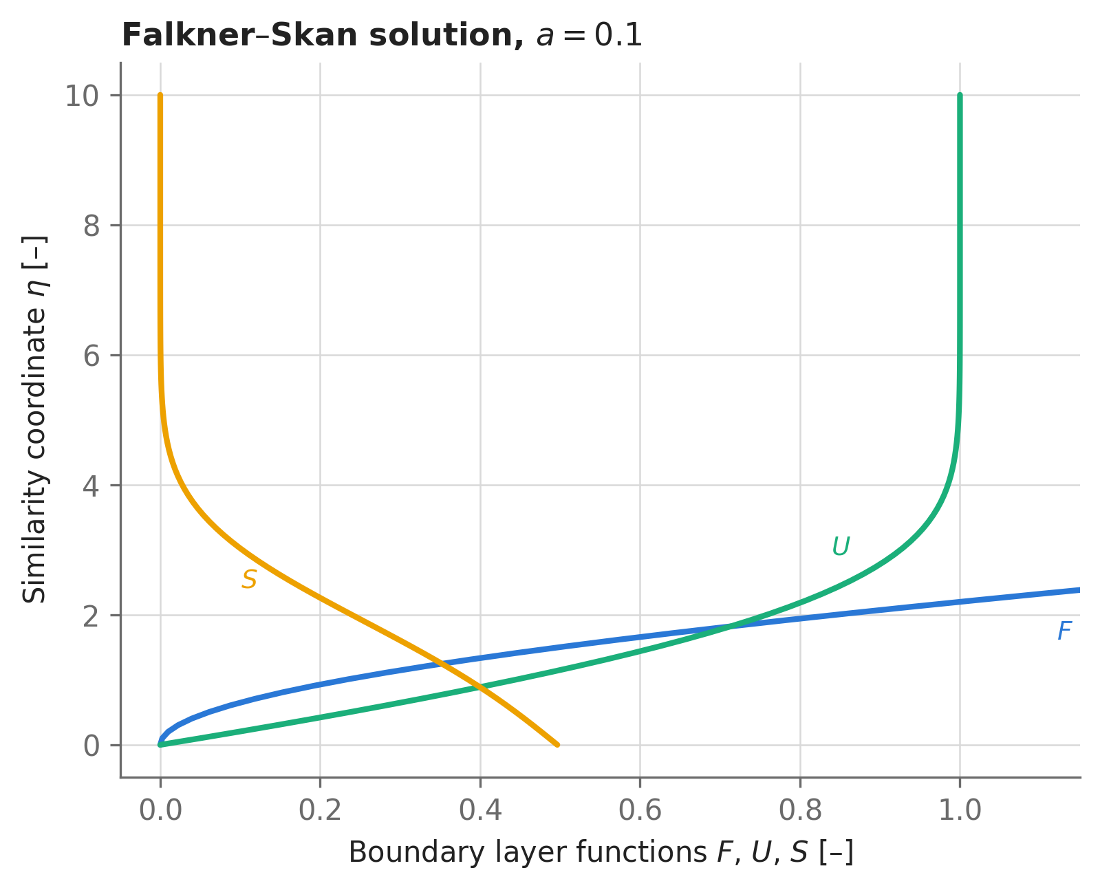
No objective was declared, so this is a pure feasibility problem: IPOPT just finds state histories satisfying all constraints — i.e., it solves the ODE. (More on feasibility problems in Chapter 5.) The wall shear parameter comes out as \(S(0) =\) 0.4965, matching the classical tabulated Falkner–Skan value for \(a = 0.1\).
Figure 12.2: Falkner–Skan solution for \(a = 0.1\), plotted in boundary-layer convention (wall at the bottom, \(\eta\) increasing upward). \(U\) is the velocity profile, \(S\) the shear profile, and \(F\) the streamfunction (which continues growing off-plot).
Because a was declared as an opti.parameter(), we can sweep it without rebuilding the problem — just opti.set_value() and re-solve. Each solve takes milliseconds:
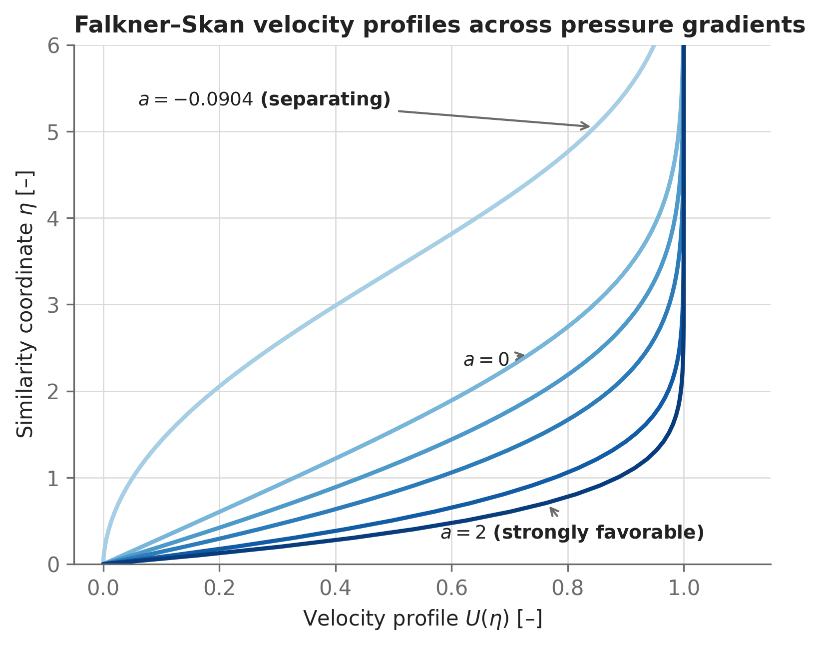
Figure 12.3: The Falkner–Skan family of velocity profiles. Favorable pressure gradients (larger \(a\), darker) produce full, separation-resistant profiles; the \(a = 0\) member is the classical Blasius flat-plate profile; adverse gradients starve the wall region of momentum until, at \(a \approx -0.0904\), the wall shear reaches zero.
12.2.1 Inverse problems come free
Look at the leftmost profile above. Its slope at the wall — the wall shear \(S(0)\) — is going to zero: this is incipient separation. The value \(a = -0.0904\) was found by trial and error. But suppose we ask the question directly: at exactly what \(a\) does the flow separate?
With a marching solver, this inverse question is painful — you’d wrap the whole ODE solve in a root-finder, and worse, for \(a\) below the critical value no solution exists, so the root-finder keeps stepping into territory where the inner solve diverges. With the simultaneous approach, the inverse problem is a two-line edit: promote a from a parameter to a variable, and add the separation condition as a constraint.
opti = asb.Opti()a = opti.variable(init_guess=0) # Was a parameter; now an unknown.F = opti.variable(init_guess=eta +10/3* (1- eta /10) **3)U = opti.derivative_of(F, with_respect_to=eta, derivative_init_guess=1- (1- eta /10) **2)S = opti.derivative_of(U, with_respect_to=eta, derivative_init_guess=0.2* (1- eta /10))opti.constrain_derivative( variable=S, with_respect_to=eta, derivative=-(1+ a) /2* F * S - a * (1- U**2),)opti.subject_to([ F[0] ==0, U[0] ==0, U[-1] ==1, S[0] ==0, # New: wall shear is exactly zero (incipient separation).])sol = opti.solve(verbose=False)a_sep = sol(a)print(f"Separation occurs at a = {a_sep:.6f}")
Separation occurs at a = -0.090443
The solver returns \(a =\) -0.0904, the known critical value. The count of unknowns and equations still balances — we added one unknown (\(a\)) and one equation (\(S(0)=0\)) — so this remains a square feasibility problem, and it costs the same as the forward solve. This pattern — swap which quantities are knowns and which are unknowns, without touching the physics — comes up constantly in engineering (e.g., “what angle of attack gives \(C_L = 0.5\)?”), and in the simultaneous formulation it’s always this easy.
12.3 Optimal control: the block move
Now we add an objective, which turns ODE-solving into optimal control. We start with the “block move” problem from Kelly’s paper — the simplest optimal control problem that exhibits all the structure of a real one:
A block of mass \(m = 1\) kg sits on a frictionless surface at position \(x = 0\), at rest. In exactly one second, it must be at \(x = 1\) m, again at rest. We may apply any force \(u(t)\) we like. Move the block while minimizing the control effort \(J = \int_0^1 u(t)^2 \, \mathrm{d}t\).
The unknowns are now three time histories — position, velocity, and force — where force is a control input: a free function of time for the optimizer to choose, appearing in the dynamics but not defined by them. The dynamics are just Newton’s second law. Note the pattern in code: derivative_of() builds the state chain downward from position, and constrain_derivative() closes the loop by attaching the physics (\(F = ma\)) at the bottom:
import aerosandbox as asbimport aerosandbox.numpy as npopti = asb.Opti()n_timesteps =100mass_block =1# [kg]time = np.linspace(0, 1, n_timesteps) # [s]position = opti.variable( # [m] init_guess=np.linspace(0, 1, n_timesteps) # guess: get there linearly)velocity = opti.derivative_of( # [m/s] position, with_respect_to=time, derivative_init_guess=1,)force = opti.variable( # [N] -- the control input init_guess=np.linspace(1, -1, n_timesteps), n_vars=n_timesteps,)opti.constrain_derivative( # F = ma variable=velocity, with_respect_to=time, derivative=force / mass_block,)effort = np.sum( # trapezoidal quadrature of integral(u^2 dt) np.integrate_discrete_intervals(f=force**2, x=time))opti.minimize(effort)opti.subject_to([ position[0] ==0, velocity[0] ==0, position[-1] ==1, velocity[-1] ==0,])sol = opti.solve(verbose=False)
The objective is a running integral, so we discretize it with the same trapezoidal quadrature the dynamics use, via np.integrate_discrete_intervals() (which returns the integral over each of the \(N-1\) intervals; summing gives the total).
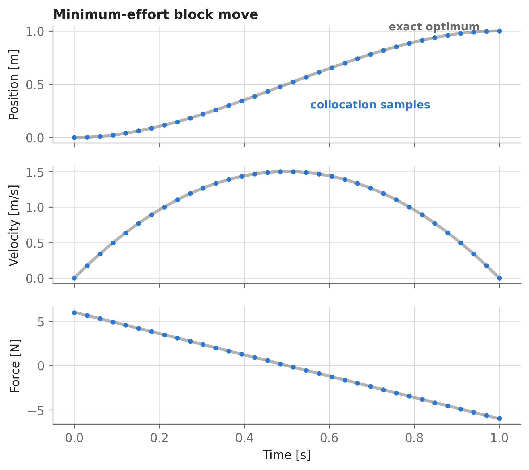
This transcribed problem has 300 variables and 202 constraints — and because the dynamics are linear and the objective quadratic, it is a quadratic program that IPOPT dispatches in 1 Newton iteration. This problem also has a known exact solution from the calculus of variations (Appendix B of Kelly’s paper): \(u^*(t) = 6 - 12t\), giving \(J^* = 12\). Our discretized solution lands at \(J =\) 12.0049 N²·s, within 0.04% of the exact optimum on this 100-point grid:
Figure 12.4: Minimum-effort block move in fixed time. The discrete collocation samples (blue dots, every 3rd shown) land on the exact calculus-of-variations optimum (gray line): a linearly decreasing force, hardest push at the start and hardest braking at the end.
NoteBoundary conditions are not initial guesses
Two distinctions that trip people up in trajectory optimization:
“Initial conditions” vs. “boundary conditions”: mathematically there is no difference — an initial condition is just a boundary condition that happens to sit at \(t = 0\). In the simultaneous formulation, position[0] == 0 and position[-1] == 1 are the same kind of object: rows in the constraint set. We use “boundary conditions” for both.
Boundary conditions vs. initial guesses: boundary conditions are constraints the solution must satisfy. Initial guesses (init_guess=) are your best estimate of the entire optimal trajectory, used only to start the Newton iteration. Good initial guesses — even crude ones, like the straight-line position profile above — dramatically improve convergence robustness.
12.4 Free final time and bang-bang control
Now for a structurally different question: what if the final time is not given, but is itself the thing to optimize? Move the block as fast as possible. As posed, that’s unbounded — with unlimited force the move takes arbitrarily little time — so we also bound the actuator: \(|u(t)| \leq 1\) N.
The formulation trick is delightfully simple. Make the final time a scalar optimization variable, and build the time grid from it:
Pause on line two: np.linspace(0, time_final, n_timesteps) is called with an optimization variable as its endpoint, and it just works — returning a symbolic vector whose spacing stretches as the solver adjusts time_final. This is the dual-backend aerosandbox.numpy from Section 2.1 earning its keep: the entire discretization is differentiable with respect to the final time, so IPOPT can reshape the time grid and the trajectory simultaneously. (The lower_bound=0 on time_final is cheap insurance against the solver exploring time running backwards.)
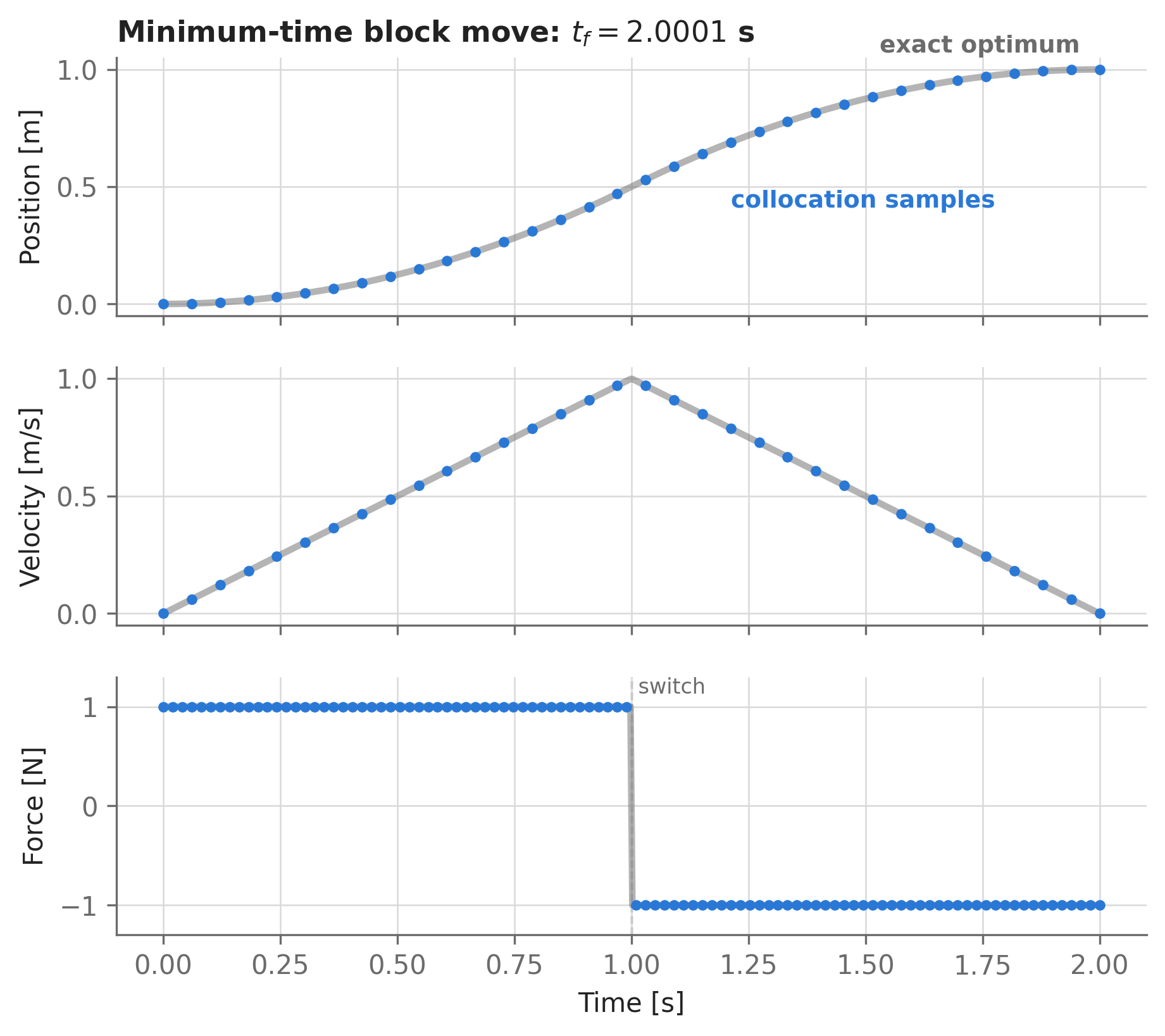
Figure 12.5: Minimum-time block move with force limited to ±1 N. The optimizer discovers bang-bang control: full throttle, then full brake, switching at the midpoint. In the force trace, every collocation sample is shown — the jump lands between two adjacent samples, so the switch instant is resolved only to within one time interval, the price of a finite grid.
The solved minimum time is \(t_f =\) 2.0001 s, against an exact answer of 2 s (accelerate at \(+1\) N for one second, brake at \(-1\) N for one second). Two things are worth savoring in this result:
Bang-bang control emerged; it was never assumed. We gave the optimizer a continuous range of admissible forces, and it discovered that the optimum lives entirely on the actuator limits. This is Pontryagin’s minimum principle in action — when the dynamics and objective are linear in a bounded control, the optimal control is bang-bang — but we never had to invoke that theory, derive costates, or guess the switching structure. For messy real-world problems (where the theory becomes intractable), the numerical approach keeps working exactly the same way.
The discontinuity is handled honestly. A discrete grid can’t place a switch at an arbitrary instant: the force samples jump from \(+1\) to \(-1\) between two adjacent grid points, so the switch time is located only to within one time interval. That’s a discretization artifact, and it shrinks as the grid refines — which brings us to the last, and arguably most important, habit of this chapter.
TipScaling free-time problems
Here the natural timescale is order-1 seconds, so time_final needed no special treatment. If your mission’s timescale is thousands of seconds (e.g., an aircraft cruise segment), give the variable a matching initial guess and consider scale= or log_transform=True — a free final time multiplies every dynamics constraint, so poor scaling on it degrades the whole problem. See Chapter 3.
12.5 Trust, but verify: refine the discretization
Every number this chapter has produced carries discretization error: we solved the transcribed problem exactly, but the transcribed problem only approximates the continuous one. Before trusting a trajectory-optimization result, always ask: does the answer stop changing as the grid refines?
Because the whole problem is just a function of the grid, this check is easy to automate — wrap the formulation in a function of \(N\) and sweep. (Notice the entire minimum-time optimal control problem fits in about a dozen lines.)
def solve_fixed_time(n):"""Minimum-effort block move on an n-point grid; returns achieved effort.""" opti = asb.Opti() time = np.linspace(0, 1, n) position = opti.variable(init_guess=np.linspace(0, 1, n)) velocity = opti.derivative_of(position, with_respect_to=time, derivative_init_guess=1) force = opti.variable(init_guess=np.linspace(1, -1, n), n_vars=n) opti.constrain_derivative(variable=velocity, with_respect_to=time, derivative=force / mass_block) effort = np.sum(np.integrate_discrete_intervals(f=force**2, x=time)) opti.minimize(effort) opti.subject_to([position[0] ==0, velocity[0] ==0, position[-1] ==1, velocity[-1] ==0])return opti.solve(verbose=False)(effort)def solve_min_time(n):"""Minimum-time block move on an n-point grid; returns achieved final time.""" opti = asb.Opti() time_final = opti.variable(init_guess=1, lower_bound=0) time = np.linspace(0, time_final, n) position = opti.variable(init_guess=np.linspace(0, 1, n)) velocity = opti.derivative_of(position, with_respect_to=time, derivative_init_guess=1) force = opti.variable(init_guess=np.linspace(1, -1, n), n_vars=n, lower_bound=-1, upper_bound=1) opti.constrain_derivative(variable=velocity, with_respect_to=time, derivative=force / mass_block) opti.subject_to([position[0] ==0, velocity[0] ==0, position[-1] ==1, velocity[-1] ==0]) opti.minimize(time_final)return opti.solve(verbose=False)(time_final)n_sweep = np.array([10, 20, 40, 80, 160, 320])error_effort = np.array([abs(solve_fixed_time(n) /12-1) for n in n_sweep])error_time = np.array([abs(solve_min_time(n) /2-1) for n in n_sweep])# Observed convergence order = -slope of the log-log error curveorder_effort =-np.polyfit(np.log(n_sweep -1), np.log(error_effort), 1)[0]order_time =-np.polyfit(np.log(n_sweep -1), np.log(error_time), 1)[0]
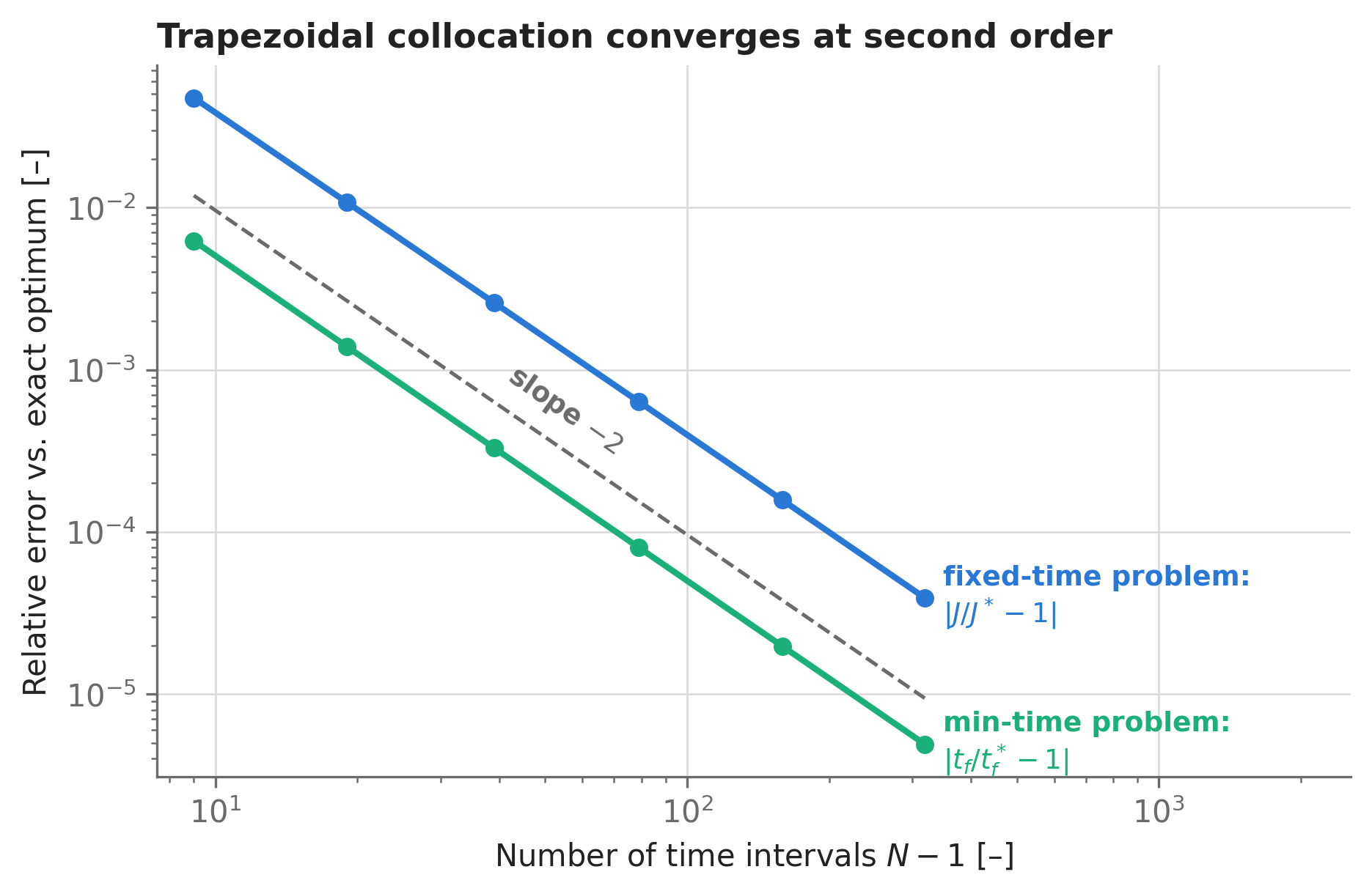
Figure 12.6: Discretization-refinement study for both block-move problems, measured against the known exact answers. Both errors fall with slope −2 on log-log axes — the signature of the second-order-accurate trapezoidal method. Since exact answers won’t exist for real problems, in practice you check that the answer stops changing between successive refinements.
The measured convergence orders are 1.99 for the fixed-time problem and 2.00 for the minimum-time problem — both the expected second-order behavior of trapezoidal collocation, even though the minimum-time control is discontinuous. (The objective converges at second order here because the switch-localization error is confined to a single shrinking interval; the reconstructed control within that interval, by contrast, is always off by order-one. Don’t expect refinement to sharpen a discontinuity — only to localize it.)
Some practical guidance that follows from this:
Work coarse, verify fine. During design iteration, 30–50 points per phase usually captures the physics and solves fast; run a refinement sweep like the one above before quoting final numbers.
Cost scales gently. Because the constraint Jacobian is sparse, doubling \(N\) roughly doubles (not quadruples) solve cost — refinement checks are cheap.
Higher-order methods pay off on smooth problems. For smooth dynamics, passing method="cubic" to derivative_of() / constrain_derivative() buys much faster convergence per grid point; for problems with switches or rough forcing, stick with the robust default.
12.6 The recipe
Every trajectory or optimal control problem in AeroSandbox follows the same six steps — and none of them required learning a new interface beyond Opti:
Grid: build a time (or space) vector — np.linspace(0, t_final, N), where t_final may itself be a variable.
States: declare the first state with opti.variable(...), and chain derived states with opti.derivative_of(...), providing honest initial guesses for each.
Controls: declare input histories as plain vector variables, with actuator limits as lower_bound= / upper_bound=.
Physics: close the loop with opti.constrain_derivative(...) — the ODE right-hand side goes here.
Boundary conditions and path constraints: ordinary opti.subject_to(...) calls on indexed states.
Objective:opti.minimize(...) — a terminal quantity, or a running integral via np.integrate_discrete_intervals(). Omit it entirely to use the machinery as a pure ODE solver.
Then solve, plot, and refine the grid until the answer stops moving.
12.7 Where to go next
Section 13.1 builds this same collocation pattern into AeroSandbox’s Dynamics classes, which write the equations of motion (point-mass and rigid-body, 2D and 3D) for you — so a full aircraft mission looks like the block move, just with better physics.
Chapter 14 uses the “everything is a constraint” mindset in space rather than time: a wing’s aerodynamics and structural deflection are coupled through shared Opti variables, giving MDO without an MDO framework.
If a trajectory solve fails or crawls, Chapter 3 covers the scaling and initial-guess hygiene that trajectory problems — with their thousands of variables — are especially sensitive to.