import aerosandbox as asb
import aerosandbox.numpy as np

N = 30  # spanwise stations on the half-wing
span = 10  # total span [m]
ys = np.linspace(0, span / 2, N)  # spanwise station locations [m]
chords = np.sqrt(np.linspace(2, 0.02, N))  # station chord lengths [m]
x_ea_over_chord = 0.40  # elastic axis location, as a fraction of chord
airfoil = asb.Airfoil("dae11")


def make_wing(heave=None, twist=None) -> asb.Wing:
    """Builds the wing in a deformed state: jig shape + heave [m] + twist [deg]."""
    if heave is None:
        heave = np.zeros(N)
    if twist is None:
        twist = np.zeros(N)

    xsecs = []
    for i in range(N):
        xyz_le = np.array([-chords[i] * x_ea_over_chord, ys[i], 0])  # jig leading edge; elastic axis at x = 0
        xyz_le = np.rotation_matrix_3D(angle=np.radians(twist[i]), axis="y") @ xyz_le  # twist about the elastic axis
        xyz_le += np.array([0, 0, heave[i]])  # then displace vertically

        xsecs.append(
            asb.WingXSec(
                xyz_le=xyz_le,
                chord=chords[i],
                twist=twist[i],
                airfoil=airfoil,
            )
        )

return asb.Wing(symmetric=True, xsecs=xsecs)14 Design Study: An Aeroelastic Wing
In this chapter, we couple a vortex-lattice aerodynamics model to a beam structural model and solve for the steady aeroelastic equilibrium of a flexible wing: the shape where the aerodynamic loads produce exactly the deformation that produces those loads. The punchline is how we couple them. There is no aero↔︎structures iteration loop, no data-transfer interface, and no multidisciplinary framework — the two disciplines simply share variables inside one asb.Opti, and IPOPT solves the coupled system in a handful of Newton iterations. With the model in hand, we then sweep airspeed to watch aeroelastic feedback amplify the loads, and extract the wing’s torsional divergence speed from first principles. The entire coupled model is roughly 80 lines of code. (This case extends an aeroelastic demonstration from the author’s PhD thesis.)
14.1 The problem: wings fight back
A wing is a spring. Build it, bolt it to a fuselage, and fly: the lift distribution bends the wing up and twists each section about its stiffness axis. But the twist changes each section’s angle of attack, which changes the lift distribution, which changes the twist… The wing you analyze on the bench (the jig shape) is not the wing that flies. For stiff, low-aspect-ratio wings the difference is a rounding error; for the flexible, high-aspect-ratio wings of sailplanes, high-altitude UAVs, and modern transports, it is a first-order effect that redistributes loads, changes total lift, and — past a critical airspeed — destroys the aircraft.
Mathematically, this is a two-discipline coupled system:
- Aerodynamics: given the deformed shape, compute the loads.
- Structures: given the loads, compute the deformation.
- Consistency: the shape the aerodynamics sees must be the jig shape plus that deformation.
The traditional approach is partitioned: run an aerodynamics code, hand the loads to a structures code, hand the deflections back, and iterate to a fixed point. This works, but it converges slowly precisely when aeroelastic effects are strong (we’ll quantify this in Section 14.7), and the plumbing between two dissimilar codes is where MDO projects go to die.
AeroSandbox invites a different, monolithic approach: declare the deformation field as optimization variables, build the aerodynamic model on the deformed geometry symbolically, write the structural governing equations as constraints, and hand the whole system to the optimizer. Because there is no objective function, this is a pure feasibility problem — a root-find on the coupled equations — and IPOPT dispatches it like Newton’s method.
14.2 A wing parameterized by its own deformation
The model wing is a tapered, unswept, symmetric wing reminiscent of a small high-altitude UAV: 10 m span, with a low-Reynolds-number DAE-11 airfoil. We describe its deformation state with two spanwise fields, sampled at N stations along the half-span:
- Heave \(u(y)\): vertical displacement of each cross-section [m], positive up.
- Twist \(\theta(y)\): rotation of each cross-section about the wing’s elastic axis [deg], positive nose-up.
The elastic axis (the axis about which a torque produces pure twist) sits at 40% chord here, typical of a wing with a mid-chord spar. Two geometry decisions make everything downstream clean:
- Put the elastic axis on the \(y\)-axis. Each section is positioned so that the point at 40% of its chord lies at \(x = 0\). Twisting a section is then simply a rotation of that section about the \(y\)-axis, and — as we’ll see — the aerodynamic torque about the elastic axis falls out of the analysis for free.
- Share one spanwise mesh. The structural stations are the aerodynamic strip boundaries, one-to-one. Coupled analyses with mismatched meshes need load-and-displacement transfer schemes; a shared mesh needs nothing.
Called with no arguments, make_wing() returns the undeformed jig shape:
import _common
import matplotlib.pyplot as plt

wing_jig = make_wing()
wing_jig.draw_three_view(style="wireframe", show=False)
plt.show()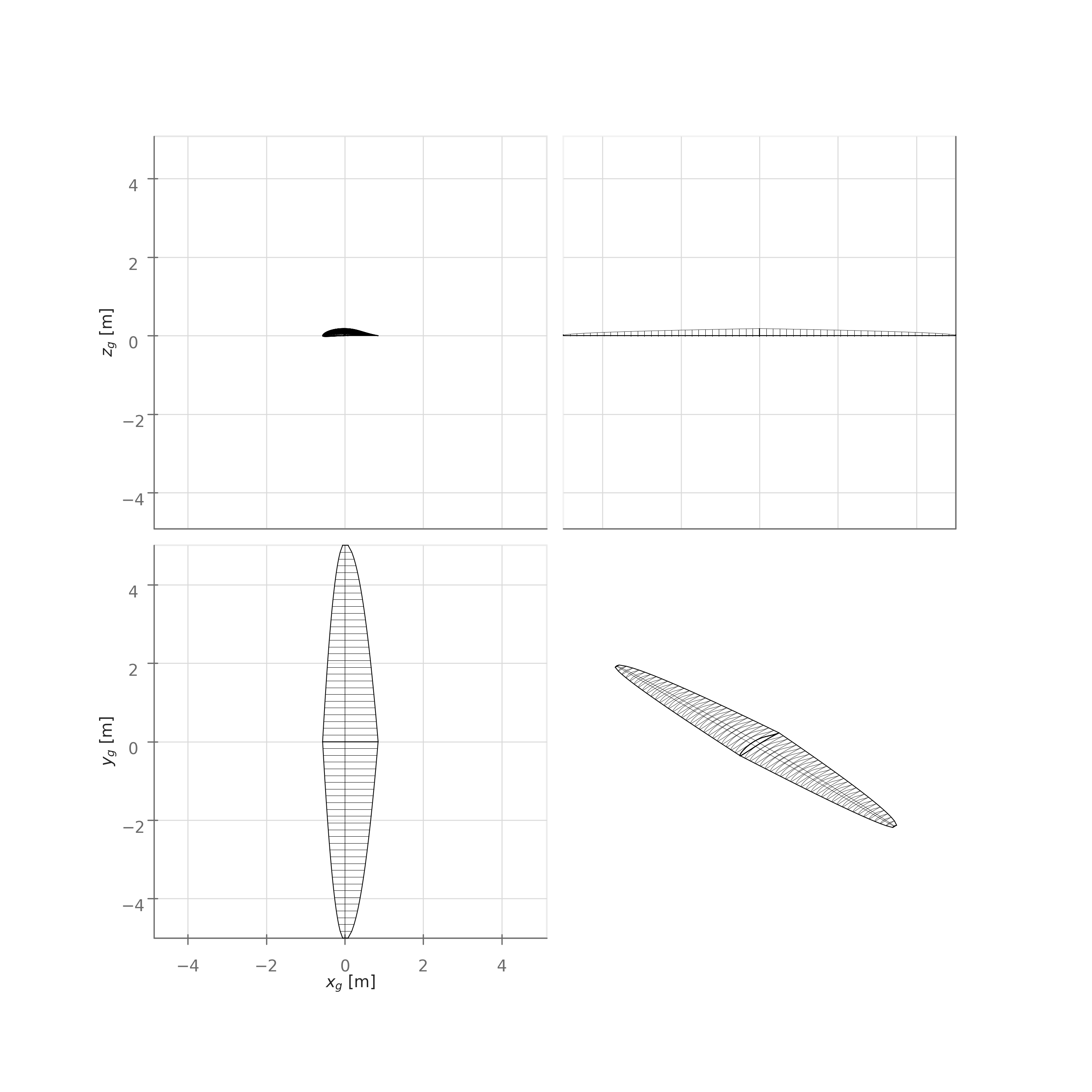
S_wing = wing_jig.area()
AR_wing = wing_jig.aspect_ratio()
print(f"Wing area:    {S_wing:.2f} m^2")
print(f"Aspect ratio: {AR_wing:.1f}")
Wing area: 9.51 m^2
Aspect ratio: 10.514.2.1 The rigid baseline
Before coupling anything, we analyze the jig shape with a standard (numeric) vortex lattice method, exactly as in Chapter 7. Two resolution choices matter:
spanwise_resolution=1keeps the VLM’s spanwise strips identical to our structural stations — the shared mesh.chordwise_resolution=1puts one chordwise panel per strip, so each strip’s lift acts at its quarter-chord line. This keeps the coupled problem small; the price is that the airfoil’s camber pitching moment is not resolved (a limitation we’ll revisit).
V_CRUISE = 10  # design flight speed [m/s]


def make_vlm(wing, velocity) -> asb.VortexLatticeMethod:
    return asb.VortexLatticeMethod(
        airplane=asb.Airplane(wings=[wing], xyz_ref=[0, 0, 0]),
        op_point=asb.OperatingPoint(velocity=velocity, alpha=5),
        spanwise_resolution=1,  # aero strips == structural stations
        chordwise_resolution=1,
    )


vlm_rigid = make_vlm(wing_jig, velocity=V_CRUISE)
aero_rigid = vlm_rigid.run()

# The VLM meshes the symmetric wing with the right half-wing's N-1 panels
# first, ordered root-to-tip. Verify, since our beam model relies on it:
assert np.all(np.diff(vlm_rigid.vortex_centers[: N - 1, 1]) > 0)

L_rigid = aero_rigid["L"]
CL_rigid = aero_rigid["CL"]
print(f"Rigid wing: L = {L_rigid:.1f} N, CL = {CL_rigid:.3f}")
Rigid wing: L = 259.4 N, CL = 0.445Because a VLM is a linear aerodynamic model, the rigid wing’s \(C_L\) is independent of airspeed — a fact we’ll lean on later when we normalize the flexible results.
14.3 The structure: a beam that feels the air
Structurally, the wing is a cantilever beam clamped at the centerline. To find the internal loads at any spanwise station, make an imaginary cut there and sum up everything acting outboard of the cut — that’s all static equilibrium is. Our aerodynamic loads are especially convenient for this: a VLM represents the lift as a set of discrete point forces \(F_j\) (one per panel, acting at the panel’s bound vortex, at spanwise location \(y^c_j\)), so the outboard sums are exact — no quadrature error:
\[ S_i = \sum_{j \ge i} F_j, \qquad M_i = \sum_{j \ge i} F_j \left( y^c_j - y_i \right), \qquad T_i = \sum_{j \ge i} \tau_j, \]
where \(S_i\), \(M_i\), and \(T_i\) are the vertical shear force [N], flapwise bending moment [N·m], and elastic-axis torque [N·m] carried by the structure at station \(y_i\), and \(\tau_j\) is the torque contributed by panel \(j\) about the elastic axis. Because we placed the elastic axis on the \(y\)-axis and set the aerodynamic moment reference to the origin, \(\tau_j\) is available directly as the \(y\)-component of the VLM’s per-panel moments — no lever-arm bookkeeping required.
The deformation then follows from the classical stiffness relations, applied station-by-station. In words: local curvature is proportional to local bending moment (Euler–Bernoulli), and local twist rate is proportional to local torque (St. Venant):
\[ EI(y) \, \frac{\mathrm{d}^2 u}{\mathrm{d} y^2} = M(y), \qquad GJ(y) \, \frac{\mathrm{d} \theta}{\mathrm{d} y} = T(y), \]
with clamped-root boundary conditions \(u(0) = 0\), \(u'(0) = 0\), \(\theta(0) = 0\). Free-tip conditions are automatic: \(M\) and \(T\) vanish at the tip because nothing is outboard of it.
For stiffness, we prescribe \(EI\) and \(GJ\) proportional to local chord cubed — what you’d get from a tube spar of constant wall thickness whose diameter scales with the chord (see Chapter 9 for sizing real spars):
EI = 2e4 * chords**3  # flapwise bending stiffness [N m^2]
GJ = 1e3 * chords**3  # torsional stiffness [N m^2]
These magnitudes are deliberately soft — a torsionally compliant wing, EI/GJ ratio of 20 — so that aeroelastic effects are clearly visible at low airspeed. The physics scales: a stiffer wing shows the same behavior at higher dynamic pressure.
One more piece of physics is worth stating before we solve, because it predicts the answer’s sign. In a VLM each strip’s lift acts at the quarter-chord; our elastic axis is at 40% chord, behind it. Lift acting ahead of the elastic axis torques the section nose-up, which raises that section’s angle of attack, which raises its lift. This positive feedback — wash-in — is the torsional divergence mechanism, and it means the flexible wing should twist nose-up and lift more than the rigid analysis predicts. (On swept-back wings, bending-induced washout typically reverses the sign — one reason sweep and aeroelasticity are so entangled.)
14.4 Closing the loop: one Opti, two disciplines
Now the coupling. We declare the deformation fields as optimization variables and build the wing — and the entire VLM analysis — on top of them. Because every AeroSandbox analysis is written in aerosandbox.numpy, the VLM traces symbolically through CasADi: aero below is not a table of numbers but a set of expressions for the loads as differentiable functions of u and theta. We also declare the airspeed as a parameter, so we can re-solve at other airspeeds later without rebuilding anything (the sweep pattern from Chapter 3).
opti = asb.Opti()

u = opti.variable(init_guess=np.zeros(N))  # heave displacement [m]
theta = opti.variable(init_guess=np.zeros(N))  # twist displacement [deg]
velocity = opti.parameter(value=V_CRUISE)  # airspeed [m/s]

vlm = make_vlm(make_wing(heave=u, twist=theta), velocity=velocity)
aero = vlm.run()  # symbolic: loads as functions of (u, theta)
Next, the internal loads. vlm.forces_geometry holds each panel’s force vector [N] in geometry axes, and vlm.moments_geometry holds each panel’s moment [N·m] about our reference at the origin — whose \(y\)-component is exactly the torque about the elastic axis. The outboard sums become a single matrix multiply against a constant 0/1 “outboard-of-this-station” matrix:
Fz = vlm.forces_geometry[: N - 1, 2]  # panel vertical forces, right half-wing [N]
tau = vlm.moments_geometry[: N - 1, 1]  # panel torques about the elastic axis [N m]
y_panel = vlm.vortex_centers[: N - 1, 1]  # panel load locations [m]

outboard = (np.arange(N - 1)[None, :] >= np.arange(N)[:, None]).astype(float)  # [i, j]: 1 if panel j is outboard of station i

S = outboard @ Fz  # shear at each station [N]
M = outboard @ (Fz * y_panel) - ys * S  # bending moment at each station [N m]
T = outboard @ tau  # torque at each station [N m]
Finally, the stiffness relations, discretized with the same trapezoidal-integration machinery used for trajectory optimization in Chapter 11: derivative_of() introduces the slope \(u'\) as a new variable tied to \(u\), and constrain_derivative() pins a variable’s derivative to a given expression.
du = opti.derivative_of(u, with_respect_to=ys, derivative_init_guess=np.zeros(N))

opti.constrain_derivative(  # Euler-Bernoulli: d(du)/dy = M / EI
    variable=du, with_respect_to=ys, derivative=M / EI
)
opti.constrain_derivative(  # St. Venant: d(theta)/dy = T / GJ, in degrees
    variable=theta, with_respect_to=ys, derivative=np.degrees(T / GJ)
)

opti.subject_to([  # clamped at the root (centerline symmetry)
    u[0] == 0,
    du[0] == 0,
    theta[0] == 0,
])
[MX(fabs(opti0_lam_g_4)), MX(fabs(opti0_lam_g_5)), MX(fabs(opti0_lam_g_6))]Note what we did not write: opti.minimize(...). With no objective, this is a feasibility problem — find any point satisfying the constraints — which is precisely what “solve the coupled aerostructural equations” means. Solve it:
sol = opti.solve()This is Ipopt version 3.14.11, running with linear solver MUMPS 5.4.1.
Number of nonzeros in equality constraint Jacobian...: 3657
Number of nonzeros in inequality constraint Jacobian.: 0
Number of nonzeros in Lagrangian Hessian.............: 1830
Total number of variables............................: 90
variables with only lower bounds: 0
variables with lower and upper bounds: 0
variables with only upper bounds: 0
Total number of equality constraints.................: 90
Total number of inequality constraints...............: 0
inequality constraints with only lower bounds: 0
inequality constraints with lower and upper bounds: 0
inequality constraints with only upper bounds: 0
iter objective inf_pr inf_du lg(mu) ||d|| lg(rg) alpha_du alpha_pr ls
0 0.0000000e+00 7.08e-02 0.00e+00 0.0 0.00e+00 - 0.00e+00 0.00e+00 0
1 0.0000000e+00 5.04e-04 0.00e+00 -11.0 1.72e+00 - 1.00e+00 1.00e+00h 1
2 0.0000000e+00 4.30e-10 0.00e+00 -11.0 7.91e-03 - 1.00e+00 1.00e+00h 1
Number of Iterations....: 2
(scaled) (unscaled)
Objective...............: 0.0000000000000000e+00 0.0000000000000000e+00
Dual infeasibility......: 0.0000000000000000e+00 0.0000000000000000e+00
Constraint violation....: 4.3029208321443413e-10 4.3029208321443413e-10
Variable bound violation: 0.0000000000000000e+00 0.0000000000000000e+00
Complementarity.........: 0.0000000000000000e+00 0.0000000000000000e+00
Overall NLP error.......: 4.3029208321443413e-10 4.3029208321443413e-10
Number of objective function evaluations = 3
Number of objective gradient evaluations = 3
Number of equality constraint evaluations = 3
Number of inequality constraint evaluations = 0
Number of equality constraint Jacobian evaluations = 3
Number of inequality constraint Jacobian evaluations = 0
Number of Lagrangian Hessian evaluations = 2
Total seconds in IPOPT = 1.485
EXIT: Optimal Solution Found.
solver : t_proc (avg) t_wall (avg) n_eval
nlp_f | 30.00us ( 10.00us) 27.86us ( 9.29us) 3
nlp_g | 8.42ms ( 2.81ms) 8.09ms ( 2.70ms) 3
nlp_grad_f | 56.00us ( 14.00us) 39.94us ( 9.98us) 4
nlp_hess_l | 1.07 s (535.97ms) 1.05 s (524.94ms) 2
nlp_jac_g | 399.78ms ( 99.95ms) 385.06ms ( 96.26ms) 4
total | 1.55 s ( 1.55 s) 1.49 s ( 1.49 s) 1n_iters = sol.stats()["iter_count"]
tip_heave = sol(u)[-1]
tip_twist = sol(theta)[-1]
CL_flex = sol(aero["CL"])
L_flex = sol(aero["L"])
amp_cruise = CL_flex / CL_rigid
print(f"Converged in {n_iters} iterations ({opti.nx} unknowns, {opti.ng} equations)")
print(f"Tip twist: {tip_twist:+.2f} deg (nose-up: wash-in, as predicted)")
print(f"Tip heave: {tip_heave:.3f} m ({tip_heave / (span / 2) * 100:.1f}% of semispan)")
print(f"Lift: {L_flex:.1f} N flexible vs. {L_rigid:.1f} N rigid ({(amp_cruise - 1) * 100:+.1f}%)")Converged in 2 iterations (90 unknowns, 90 equations)
Tip twist: +1.71 deg (nose-up: wash-in, as predicted)
Tip heave: 0.050 m (1.0% of semispan)
Lift: 304.1 N flexible vs. 259.4 N rigid (+17.3%)Read that iteration count again. IPOPT solved the fully-coupled aeroelastic system — a 90-unknown nonlinear root-find where every residual depends on a vortex-lattice solve — in 2 Newton steps, because it has exact derivatives of everything with respect to everything. There is no “aeroelastic iteration” anywhere in the code above.
The headline number: at a flight speed of just 10 m/s, flexibility increases this wing’s lift by 17%. A rigid-wing analysis of this airplane wouldn’t just be slightly off — it would mis-predict trim, loads, and performance across the board.
14.5 What flexibility does to the loads
The spanwise picture tells the story. The nose-up twist builds from root to tip (torque accumulates inboard, but stiffness falls off outboard as \(c^3\)), so the outboard wing gains the most angle of attack — and the lift distribution shifts outboard accordingly.
import _common

y_panel_num = vlm_rigid.vortex_centers[: N - 1, 1]  # panel load locations [m]
dy = np.diff(ys)  # panel widths [m]
lift_rigid = vlm_rigid.forces_geometry[: N - 1, 2] / dy  # [N/m]
lift_flex = sol(Fz) / dy  # [N/m]

fig, ax = plt.subplots(3, 1, sharex=True, figsize=(7, 7.5))

ax[0].plot(y_panel_num, lift_rigid, color="gray")
ax[0].plot(y_panel_num, lift_flex, color=_common.SERIES[0])
i_label = N // 2
_common.label_line(ax[0], y_panel_num[i_label], lift_rigid[i_label], "rigid (jig shape)", "gray", dy=-7)
_common.label_line(ax[0], y_panel_num[i_label], lift_flex[i_label], "flexible", _common.SERIES[0], dy=3)
ax[0].set_ylabel("Lift per unit span [N/m]")
ax[0].set_title("Flexibility shifts the lift distribution outboard")

ax[1].plot(ys, sol(theta), color=_common.SERIES[0])
ax[1].axhline(0, color="gray", linewidth=0.8)
ax[1].set_ylabel("Twist $\\theta$ [deg]")
ax[1].set_title("Nose-up twist (wash-in) accumulates toward the tip")

ax[2].plot(ys, sol(u), color=_common.SERIES[0])
ax[2].set_ylabel("Heave $u$ [m]")
ax[2].set_title("Bending deflection")
ax[2].set_xlabel("Spanwise position $y$ [m]")

plt.tight_layout()
plt.show()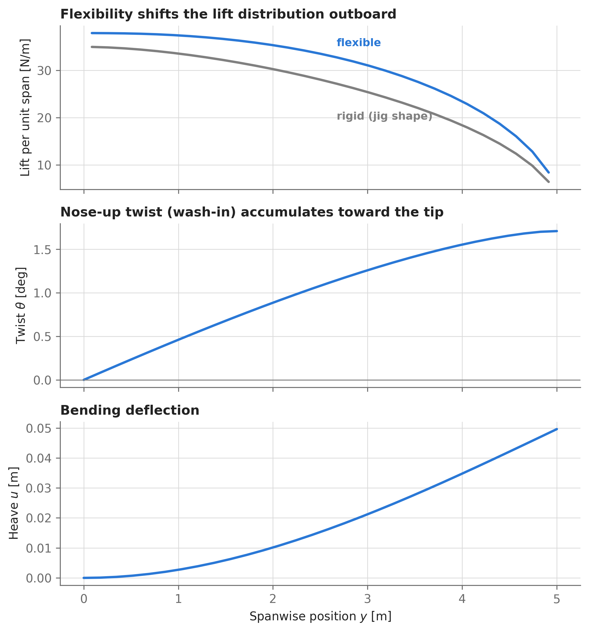
The structural half of the answer comes for free: the same M and T expressions we constrained are, at the solution, the design loads you would hand to a spar-sizing analysis (Chapter 9). Note the double penalty relative to a rigid loads analysis: the flexible wing carries more total lift, and carries it further outboard — both of which raise the root bending moment.
import _common

root_M = sol(M)[0]
root_T = sol(T)[0]

fig, ax = plt.subplots(2, 1, sharex=True, figsize=(7, 5))

ax[0].plot(ys, sol(M), color=_common.SERIES[3])
_common.label_line(ax[0], ys[0], root_M, f"  root: {root_M:.0f} N·m", _common.SERIES[3], dx=0.15)
ax[0].set_ylabel("Bending moment $M$ [N·m]")
ax[0].set_title("Bending moment, flexible wing")

ax[1].plot(ys, sol(T), color=_common.SERIES[4])
_common.label_line(ax[1], ys[0], root_T, f"  root: {root_T:.1f} N·m", _common.SERIES[4], dx=0.15)
ax[1].set_ylabel("Torque $T$ [N·m]")
ax[1].set_title("Elastic-axis torque, flexible wing")
ax[1].set_xlabel("Spanwise position $y$ [m]")

plt.tight_layout()
plt.show()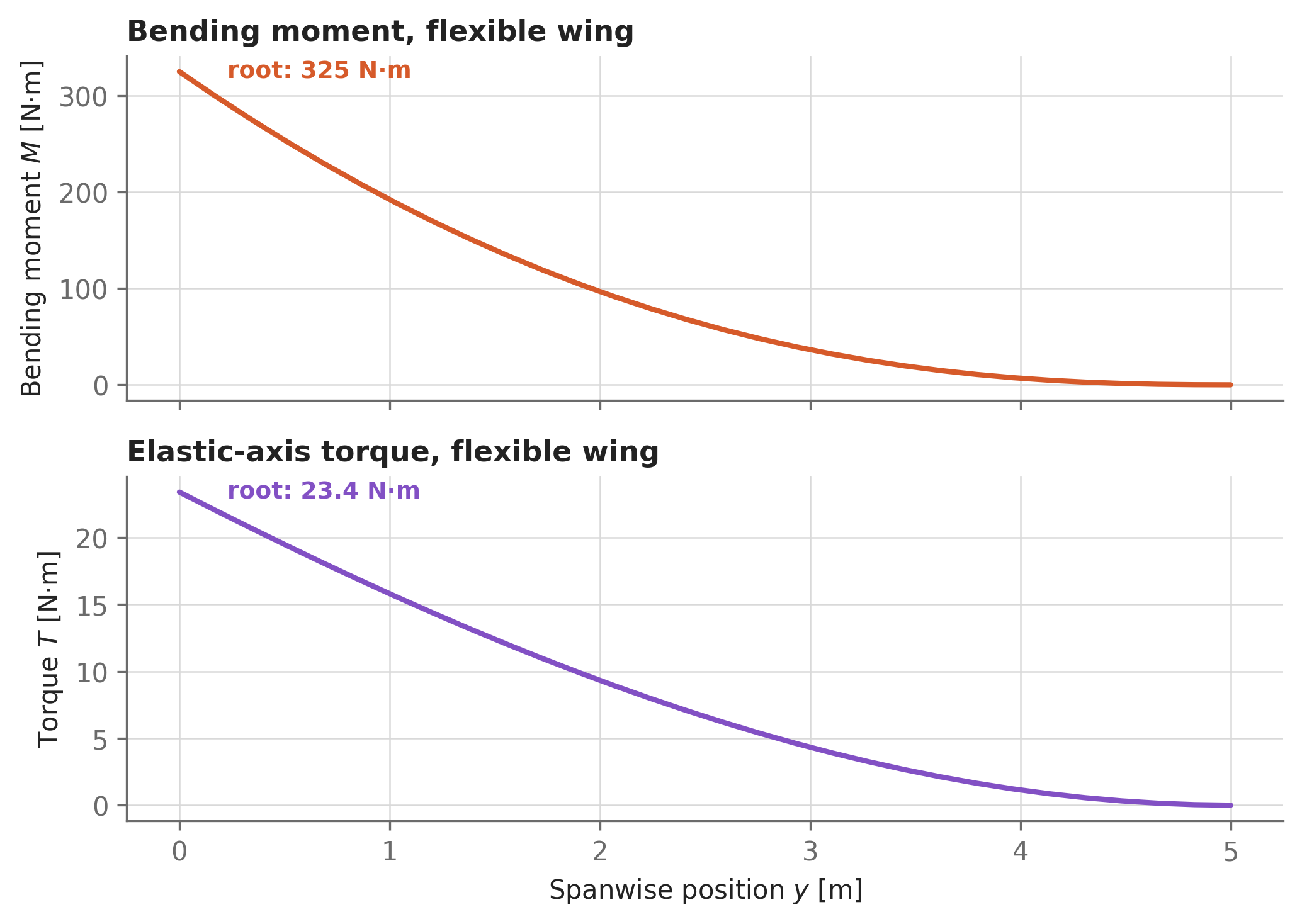
14.6 Flying faster: the road to torsional divergence
Why does flexibility amplify lift here, and what sets the limit? Walk the feedback loop once: a twist increment raises lift; the extra lift, acting ahead of the elastic axis, produces extra nose-up torque proportional to dynamic pressure \(q\); the structure yields additional twist proportional to that torque. Each trip around the loop multiplies the previous twist increment by a gain \(g \propto q\) (the aerodynamic torque scales with \(q\); the structural stiffness doesn’t care about airspeed). Summing the geometric series, the equilibrium lift amplification is
\[ A(q) \;=\; \frac{L_\text{flexible}}{L_\text{rigid}} \;=\; 1 + g + g^2 + \cdots \;=\; \frac{1}{1 - q/q_\text{div}}, \]
where \(q_\text{div}\) is the dynamic pressure at which the gain reaches one and the series — and the wing — diverges. This single-mode model makes a sharp, testable prediction: \(1/A\) should fall linearly with \(q\), hitting zero at \(q_\text{div}\).
Let’s test it against the full coupled model. Because velocity is a parameter, each new flight condition is a parameter_mapping away — same problem, same symbolic graph, new number — and we warm-start each solve from the previous solution:
V_sweep = [6, 12, 15, 18, 20]  # airspeeds to add to our 10 m/s solution [m/s]

V_all = [V_CRUISE]
CL_all = [CL_flex]
tip_twist_all = [tip_twist]

sol_V = sol
for V in V_sweep:
    opti.set_initial_from_sol(sol_V)  # warm start from the previous equilibrium
    sol_V = opti.solve(parameter_mapping={velocity: V}, verbose=False)

    V_all.append(V)
    CL_all.append(sol_V(aero["CL"]))
    tip_twist_all.append(sol_V(theta)[-1])
    print(f"V = {V:2d} m/s: CL = {CL_all[-1]:.3f}, tip twist = {tip_twist_all[-1]:5.2f} deg")
V = 6 m/s: CL = 0.470, tip twist = 0.55 deg
V = 12 m/s: CL = 0.565, tip twist = 2.67 deg
V = 15 m/s: CL = 0.666, tip twist = 4.93 deg
V = 18 m/s: CL = 0.847, tip twist = 8.89 deg
V = 20 m/s: CL = 1.070, tip twist = 13.65 degThe twist growth is clearly super-linear in airspeed. Now the divergence-model check — fit a line to \(1/A\) versus \(q\) and extrapolate to zero:
order = np.argsort(V_all)
V_arr = np.array(V_all)[order]
amp_arr = np.array(CL_all)[order] / CL_rigid  # lift amplification A [-]
tip_twist_arr = np.array(tip_twist_all)[order]

rho = vlm_rigid.op_point.atmosphere.density()  # air density [kg/m^3]
q_arr = 0.5 * rho * V_arr**2  # dynamic pressure [Pa]

slope, intercept = np.polyfit(q_arr, 1 / amp_arr, 1)
q_div = -intercept / slope  # dynamic pressure where 1/A -> 0 [Pa]
V_div = np.sqrt(2 * q_div / rho)  # divergence speed [m/s]

print(f"Fit intercept: {intercept:.3f}   (single-mode theory predicts 1)")
print(f"Extrapolated divergence: q_div = {q_div:.0f} Pa  ->  V_div = {V_div:.1f} m/s")
Fit intercept: 0.998 (single-mode theory predicts 1)
Extrapolated divergence: q_div = 419 Pa -> V_div = 26.2 m/sThe fit intercept lands within a fraction of a percent of the theoretical value of 1, so the one-degree-of-freedom feedback model captures this wing’s aeroelasticity almost perfectly — a satisfying case of a one-line geometric-series argument agreeing with a 90-unknown coupled simulation:
import _common

fig, ax = plt.subplots(2, 1, sharex=True, figsize=(7, 6))

ax[0].plot(V_arr, tip_twist_arr, "o-", color=_common.SERIES[0])
ax[0].set_ylabel("Tip twist [deg]")
ax[0].set_title("Twist runs away as airspeed rises")

V_fit = np.linspace(0, 0.92 * V_div, 300)
amp_fit = 1 / (intercept + slope * 0.5 * rho * V_fit**2)
ax[1].plot(V_fit, amp_fit, "--", color="gray", zorder=1)
ax[1].plot(V_arr, amp_arr, "o", color=_common.SERIES[0], zorder=2)
_common.label_line(ax[1], V_arr[2], amp_arr[2], "coupled model", _common.SERIES[0], dx=0.3, dy=-0.6)
_common.label_line(ax[1], V_fit[270], amp_fit[270], "$A = 1/(1 - q/q_\\mathrm{div})$", "gray", dx=-9)
ax[1].set_ylim(0, None)
_common.annotate_event(ax[1], V_div, f"$V_\\mathrm{{div}}$ = {V_div:.1f} m/s")
ax[1].set_ylabel("Lift amplification $L_\\mathrm{flex}/L_\\mathrm{rigid}$ [-]")
ax[1].set_xlabel("Airspeed $V$ [m/s]")
ax[1].set_title("Lift amplification follows the divergence law")

plt.tight_layout()
plt.show()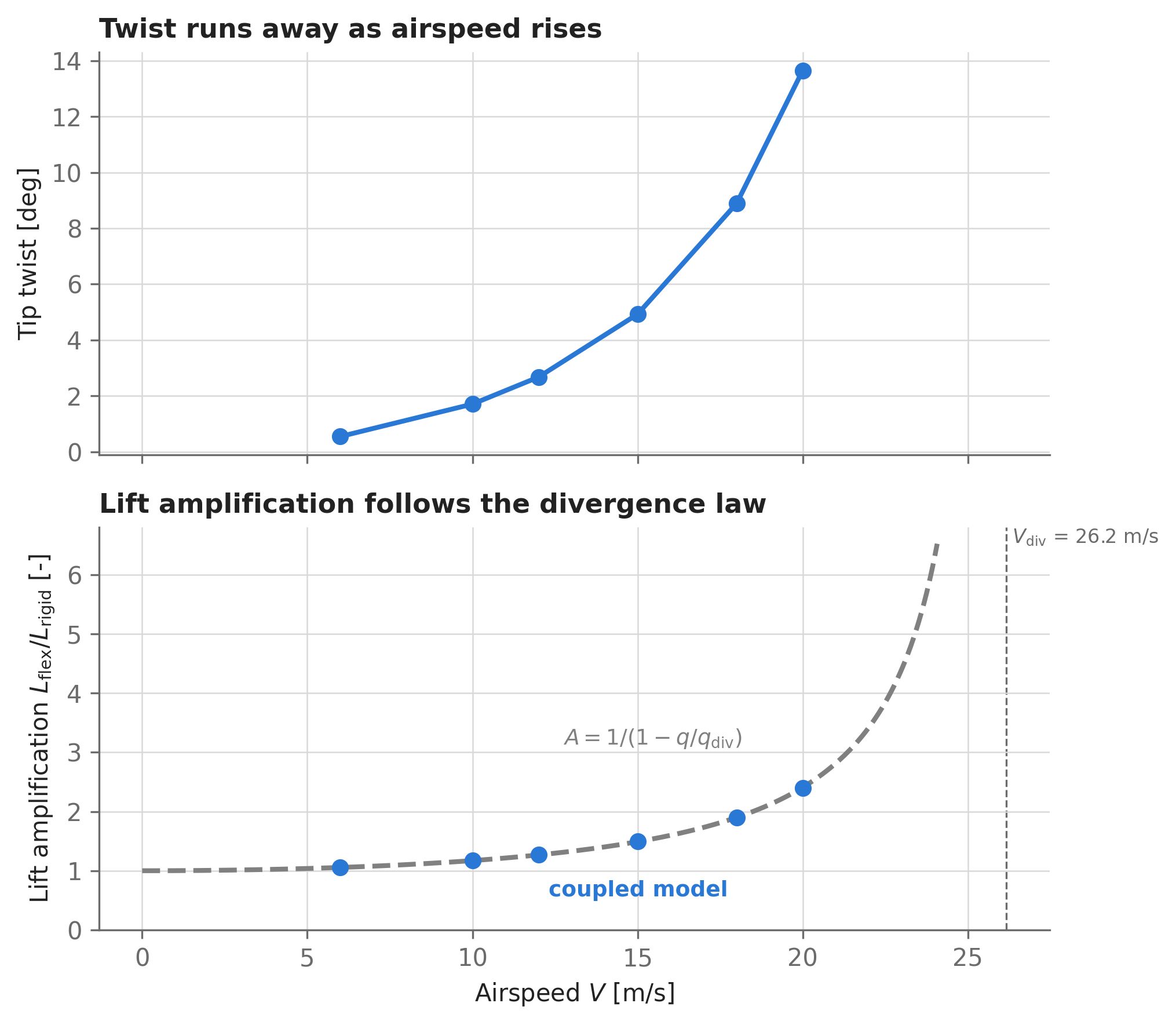
At the top of our sweep — twice the design flight speed, but still well below \(V_\text{div}\) — the deformation is anything but subtle:
import _common

wing_deformed = make_wing(heave=sol_V(u), twist=sol_V(theta))
wing_deformed.color = _common.SERIES[0]
wing_jig.color = "gray"

axs = wing_jig.draw_three_view(style="wireframe", show=False)
axs = wing_deformed.draw_three_view(axs=axs, style="wireframe", show=False)
plt.show()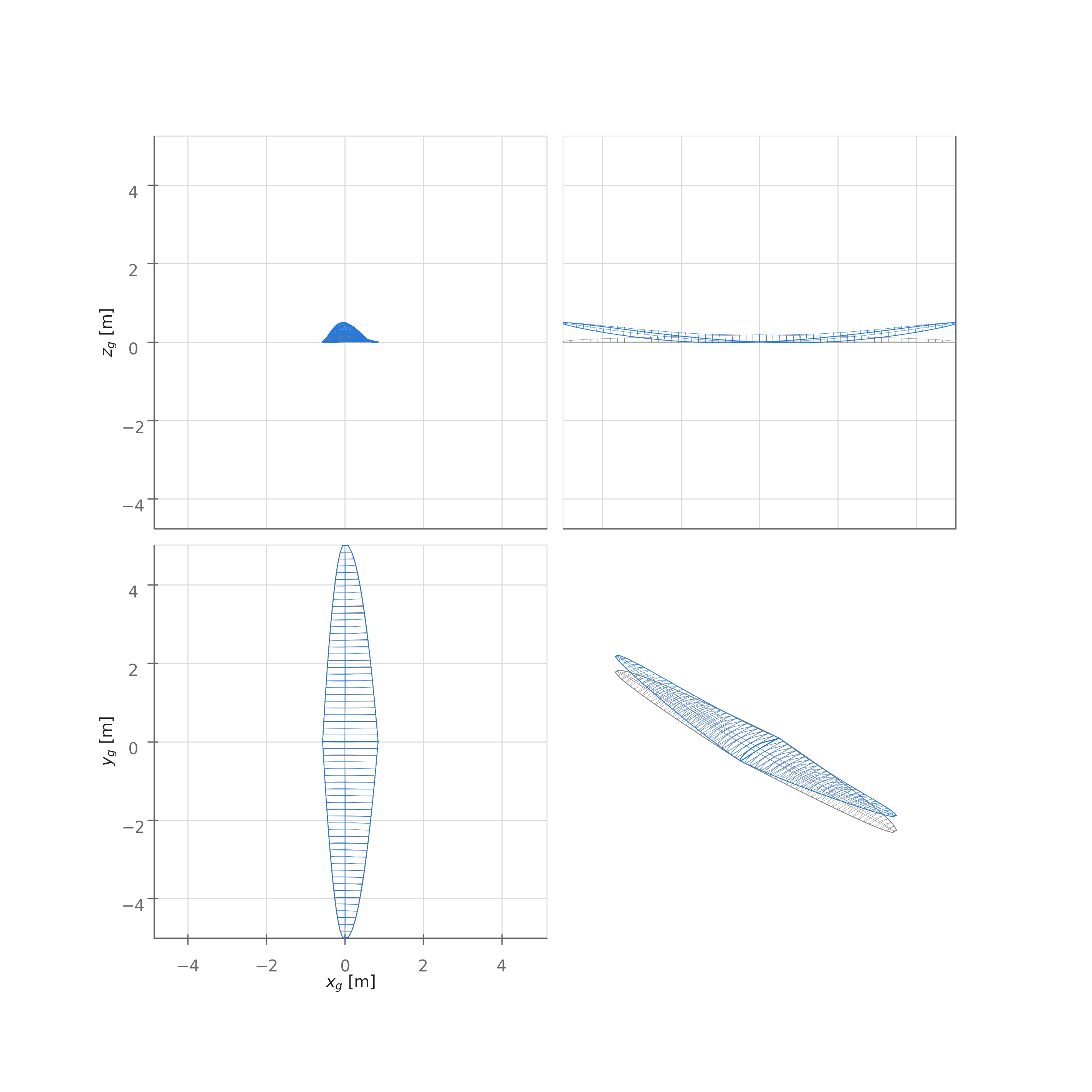
print(f"At 20 m/s: tip twist = {tip_twist_all[-1]:.1f} deg, "
      f"tip heave = {sol_V(u)[-1]:.2f} m ({sol_V(u)[-1] / (span / 2) * 100:.0f}% of semispan), "
      f"lift amplification = {amp_arr[-1]:.2f}")
At 20 m/s: tip twist = 13.7 deg, tip heave = 0.48 m (10% of semispan), lift amplification = 2.40And what if we push past the sweep? Ask for an equilibrium at 23 m/s:
V_push = 23  # [m/s]
amp_predicted = 1 / (intercept + slope * 0.5 * rho * V_push**2)  # linear theory's prediction

try:
    opti.set_initial_from_sol(sol_V)
    opti.solve(parameter_mapping={velocity: V_push}, verbose=False, max_iter=300)
except RuntimeError as e:
    print(f"Solve FAILED at V = {V_push} m/s. Solver message:")
    print("   ", str(e).splitlines()[-1])
Solve FAILED at V = 23 m/s. Solver message:
Solver failed. You may use opti.debug.value to investigate the latest values of variables. return_status is 'Infeasible_Problem_Detected'The solver searches, then reports that it converged to a point of local infeasibility: it cannot find any deformation state that satisfies both disciplines simultaneously. Here that is not a modeling bug — it is the physics talking. Near divergence, equilibria become extreme (the linear fit predicts a lift amplification of 4.4 at this speed) and then cease to exist; the honest operational conclusion is simply do not fly this wing that fast. Two caveats deserve mention. First, “locally infeasible” is a local statement — the failed-solve decision tree in the FAQ appendix covers how to distinguish physics from poor initial guesses. Second, our extrapolated \(V_\text{div}\) comes from linear, small-displacement theory; the nonlinear coupled model starts losing equilibria somewhat earlier, so the linear number should be read as an upper bound.
14.7 MDO without an MDO framework
Step back and inventory what the coupling cost us:
- Zero interface code. The disciplines communicate through shared
Optivariables (u,theta) and shared expressions (Fz,tau). There is no load-transfer module, no file format, no framework API — the “data exchange” is CasADi’s expression graph. - Zero outer iteration. A partitioned aero↔︎structures loop is a fixed-point iteration whose error contracts by roughly the feedback gain \(q/q_\text{div}\) per pass — so at 90% of divergence it needs dozens of passes, each one a full aero solve, and at divergence it never converges. The monolithic Newton approach solved every point in our sweep in a handful of iterations, with cost essentially independent of how strong the coupling is.
- A few matrix multiplies of structural code. The beam model — internal loads by free-body cut, plus two stiffness constraints — is about fifteen lines.
This is the general AeroSandbox pattern for multidisciplinary analysis: make the coupling variables optimization variables, write each discipline’s governing equations as constraints, and let the optimizer own the convergence loop. It scales far past two disciplines — the design studies in Chapter 14 and Chapter 15 couple aerodynamics, structures, propulsion, weights, and energy models in exactly this way.
It also converts analysis into design almost for free. Everything above had no objective function; add one, promote a few model constants to variables, and the same coupled physics becomes an aerostructural optimization — no new machinery:
# Sketch: from analysis to design (not run here)
jig_twist = opti.variable(init_guess=np.zeros(N))  # washout distribution becomes a design variable
# ... build make_wing() with twists = jig_twist + theta ...
opti.subject_to(aero["L"] >= W)  # lift the airplane's weight
opti.minimize(aero["D"])  # minimize drag of the *flying* (deformed) shape
The optimizer then shapes the jig so that the deformed wing is optimal — which is, after all, the wing the airplane actually flies.
Honesty requires listing what this demonstration model leaves out: it is a linear, small-displacement beam (strained by the largest deflections shown here); torque is taken about the undeformed elastic axis; the single-chordwise-panel VLM omits the airfoil’s camber pitching moment and, being inviscid, will never stall no matter how much wash-in develops; the elastic axis is unswept, so sweep-induced bend-twist coupling is absent; and the analysis is static — flutter, the dynamic aeroelastic instability, needs unsteady aerodynamics entirely outside this model’s scope. Every one of these is a modeling upgrade, not an architectural one: each slots into the same Opti as more expressions and constraints.
14.8 Where to go next
- Chapter 9 shows how to compute realistic
EIandGJdistributions from actual spar geometry — swap those in for the prescribed stiffness used here, and add spar mass to close the loop with weights. - Chapter 3 covers the parameter/warm-start sweep machinery used here, plus what to do when a solve fails.
- Chapter 14 applies this chapter’s coupling philosophy to a full transport-aircraft sizing problem — the “complete design study” version of the pattern.