import aerosandbox as asb
import aerosandbox.numpy as np
from aerosandbox.tools import units as u

opti = asb.Opti()

### Mission definition
n_pax = 400
mach_cruise = 0.82
altitude_cruise = 35e3 * u.foot

mission_range = opti.parameter(value=7500 * u.naut_mile)

### Fuel properties, as parameters so we can swap fuels later without re-tracing.
# LH2 values from Brewer, "Hydrogen Aircraft Technology", pg. 203.
fuels = {
    "Jet A": dict(
        density=820,  # kg/m^3
        specific_energy=43.02e6,  # J/kg, lower heating value
        tank_fuel_mass_fraction=0.993,  # m_fuel / (m_fuel + m_tank)
        tank_wall_thickness=0.005,  # m
        system_mass_multiplier=1.0,  # fuel lines, pumps
    ),
    "LH2": dict(
        density=70,
        specific_energy=119.93e6,
        tank_fuel_mass_fraction=1 / (1 + 0.356),  # insulated cryogenic tank
        tank_wall_thickness=0.0612,  # includes insulation
        system_mass_multiplier=2.2,  # cryo pumps, vent lines
    ),
}

fuel = {k: opti.parameter(value=v) for k, v in fuels["Jet A"].items()} # Jet A baseline15 Design Study: A Long-Range Transport Aircraft
16 Design Study: A Long-Range Transport Aircraft
This chapter sizes a complete 400-passenger, 7,500-nautical-mile transport aircraft — a 777-class twinjet — as a single optimization problem. Geometry, cruise aerodynamics (via asb.AeroBuildup), rubber-engine propulsion, a Raymer/TASOPT-style weight buildup, and mission performance all close simultaneously: no sizing loops, no fixed-point iteration, no MDO framework. You will learn how to structure a multidisciplinary sizing model so that it solves reliably (positivity by construction, NaN-safe reformulations, normalized constraints), and how to reuse one traced model for many design questions — including the headline stunt: converting the airplane from Jet A to liquid hydrogen by changing five numbers, then re-solving in seconds.
This model is distilled from the lh2_airplane.py study in the AeroSandbox repository (studies/SimulateAeroBuildupTrajectory/), pruned to its didactic core.
16.1 The design problem
The mission: carry 400 passengers 7,500 nautical miles at Mach 0.82, cruising at 35,000 ft, with two engines. That is roughly the design mission of a Boeing 777-300ER or 777-9, which gives us something rare and valuable in conceptual design: a published answer key.
The classic way to size such an aircraft is a sizing loop: guess a takeoff gross weight (TOGW), size the wing and engines to it, compute the fuel required, add up the weights, get a new TOGW, and iterate until the numbers stop moving. The optimization-native way is to instead declare TOGW as a design variable and write the loop’s convergence condition as a constraint:
\[ \underbrace{m_\text{empty} + m_\text{payload} + m_\text{fuel}}_{\text{what the airplane adds up to}} \leq \underbrace{m_\text{TOGW}}_{\text{what everything was sized to}} \]
The optimizer then closes the loop and optimizes the design in the same breath. Here is the full problem we will pose:
| Role | Quantity | Notes |
|---|---|---|
| Minimize | design takeoff gross weight \(m_\text{TOGW}\) | the classic conceptual-design objective |
| With respect to | \(m_\text{TOGW}\) | log-transformed |
| wing span \(b\) | log-transformed, \(\leq 65\) m (gate limit) | |
| wing yehudi chord \(c_\text{yehudi}\) | log-transformed; root chord derived | |
| fuel tank interior length \(\ell_\text{tank}\) | log-transformed; sets fuel load | |
| cruise angle of attack \(\alpha\) | bounded ±few degrees | |
| cruise lift-to-drag handle \((L/D)\) | log-transformed helper variable | |
| Subject to | mass buildup \(\leq m_\text{TOGW}\) | weight closure |
| lift \(\geq\) weight at mid-cruise | vertical force balance | |
| Breguet range \(\geq\) mission range | fuel closure (NaN-safe form) | |
| \((L/D) \cdot C_D \leq C_L\) | ties the handle to the aero analysis | |
| approach speed \(\leq\) 145 kn | field performance | |
| Parameters | mission range; fuel properties (5 numbers) | swappable without re-tracing |
Everything else — fuselage cabin dimensions (set by the passenger count), wing sweep, cruise Mach and altitude, tail geometry, engine count — is frozen at 777-like values. We will be explicit about those freezes and what it would take to relax them in Section 16.11.
16.2 Parameters vs. variables
A decision that pays off later: quantities we intend to sweep are declared as opti.parameter() rather than baked-in constants. A parameter is a symbolic leaf in the computational graph whose value can be changed after the problem is built — so one traced model can answer many design questions, each re-solve taking seconds. (This is the same mechanism behind the design sweeps in the solvers chapter.)
Now the design variables. Every one that is physically positive gets log_transform=True. This is not a style preference — it is what makes a model this nonlinear solve reliably. A log-transformed variable is positive at every iterate, including the infeasible ones the optimizer merely passes through, so downstream expressions like \((\text{wing area})^{0.649}\) can never see a negative base. (The full argument for this, with failure modes, is in the robust-optimization-models chapter.)
design_mass_TOGW = opti.variable(init_guess=300e3, log_transform=True)  # kg

# ICAO Code E gates cap the span at 65 m -- the actual reason the 777-300ER's
# span is 64.8 m (and why the 777-9 folds its wingtips). Without this bound,
# the optimizer runs to aspect ratios no airport could park.
wing_span = opti.variable(init_guess=60, log_transform=True, upper_bound=65)  # m

wing_yehudi_chord = opti.variable(init_guess=9, log_transform=True, upper_bound=20)  # m

# Interior length of EACH of the two fuselage fuel tanks. Making the *interior*
# length the variable (rather than the exterior) keeps the tank volume positive
# by construction, even at wall thicknesses the optimizer never sees.
tank_interior_length = opti.variable(init_guess=3, log_transform=True, upper_bound=20)  # m

alpha_cruise = opti.variable(init_guess=3, lower_bound=-5, upper_bound=10)  # deg
Note what is not a variable: the wing root chord. The planform has a straight inboard trailing edge (the “yehudi” of a Boeing-style wing), so the root chord is derived from the yehudi chord plus the sweep — guaranteeing every chord is positive at any iterate, with no constraint needed. As a rule: when quantity B is quantity A plus something nonnegative, make A the variable and derive B.
16.3 Geometry
We write the geometry as a plain function. Called with floats, it builds a numeric airplane we can draw; called with opti variables, it builds the symbolic airplane the optimizer sees. This backend-agnosticism is the core AeroSandbox idiom — the same code traces through CasADi or runs on NumPy (see the geometry chapter for the full Airplane stack).
### Frozen configuration constants (777-class)
cabin_diameter = 6.20  # m, twin-aisle cabin for ~400 pax
cabin_length = 37.6  # m
nose_fineness, tail_fineness = 1.67, 2.62  # length/diameter of nose, tailcone
wing_sweep_deg = 34  # leading-edge sweep
wing_dihedral_deg = 6
wing_airfoil = asb.Airfoil("b737d")  # 737 outboard transonic section, t/c ~ 10.8%
hstab_airfoil = asb.Airfoil("naca0012")
vstab_airfoil = asb.Airfoil("naca0008")


def make_airplane(wing_span, wing_yehudi_chord, tank_interior_length, tank_wall_thickness):
    """Build the airplane. Works symbolically (opti vars) or numerically (floats)."""
    cabin_radius = cabin_diameter / 2
    tank_length = tank_interior_length + 2 * tank_wall_thickness

    ### Fuselage: nose cone | fwd tank | cabin | aft tank | tail cone.
    # The tanks and cabin share one constant-radius cylinder; only the internal
    # bookkeeping distinguishes them.
    x_fwd_tank = nose_fineness * cabin_diameter  # nose ends here
    x_cabin = x_fwd_tank + tank_length
    x_aft_tank = x_cabin + cabin_length
    x_tail_start = x_aft_tank + tank_length
    x_tail_end = x_tail_start + tail_fineness * cabin_diameter

    t = np.sinspace(0, 1, 8)  # nondimensional arc coordinate for nose/tail shaping
    xf = np.concatenate([
        t * x_fwd_tank,
        np.array([x_tail_start]),
        x_tail_start + t[1:] * (x_tail_end - x_tail_start),
    ])
    zf = np.concatenate([  # centerline droop (nose) and upsweep (tail)
        -0.3 * (1 - t) ** 2 * cabin_radius,
        np.array([0]),
        t[1:] ** 1.5 * cabin_radius,
    ])
    rf = np.concatenate([
        (1 - (1 - t) ** 2) ** 0.5 * cabin_radius,
        np.array([cabin_radius]),
        (1 - t[1:] ** 1.5) * cabin_radius,
    ])

    fuselage = asb.Fuselage(
        name="Fuselage",
        xsecs=[
            asb.FuselageXSec(xyz_c=[xf[i], 0, zf[i]], radius=rf[i])
            for i in range(np.length(xf))
        ],
        analysis_specific_options={
            asb.AeroBuildup: dict(nose_fineness_ratio=nose_fineness)
        },
    )

    ### Wing: root -> yehudi (25% span) -> tip, with straight inboard trailing edge
    half_span = wing_span / 2
    yehudi_y = 0.25 * half_span
    root_chord = wing_yehudi_chord + yehudi_y * np.tand(wing_sweep_deg)

    def wing_xsec(y, chord):
        return asb.WingXSec(
            xyz_le=[y * np.tand(wing_sweep_deg), y, y * np.tand(wing_dihedral_deg)],
            chord=chord,
            airfoil=wing_airfoil,
        )

    wing = asb.Wing(
        name="Main Wing",
        symmetric=True,
        xsecs=[
            wing_xsec(0, root_chord),
            wing_xsec(yehudi_y, wing_yehudi_chord),
            wing_xsec(half_span, 0.14 * root_chord),
        ],
    ).translate([
        0.5 * (x_cabin + x_aft_tank) - 0.5 * root_chord,  # wing carries the cabin
        0,
        -0.5 * cabin_radius,  # low wing
    ])

    ### Tails: frozen 777-scale geometry, translated with the (stretchable) tailcone
    hstab = asb.Wing(
        name="Horizontal Stabilizer",
        symmetric=True,
        xsecs=[
            asb.WingXSec(xyz_le=[0, 0, 0], chord=7.0, airfoil=hstab_airfoil),
            asb.WingXSec(
                xyz_le=[10.8 * np.tand(35), 10.8, 0], chord=2.45, airfoil=hstab_airfoil
            ),
        ],
    ).translate([x_tail_end - 10.5, 0, 0.5 * cabin_radius])

    vstab = asb.Wing(
        name="Vertical Stabilizer",
        xsecs=[
            asb.WingXSec(xyz_le=[0, 0, 0], chord=7.6, airfoil=vstab_airfoil),
            asb.WingXSec(
                xyz_le=[10 * np.tand(35), 0, 10], chord=3.4, airfoil=vstab_airfoil
            ),
        ],
    ).translate([x_tail_end - 11.4, 0, cabin_radius])

    airplane = asb.Airplane(
        name="Transport",
        wings=[wing, hstab, vstab],
        fuselages=[fuselage],
    )
    stations = dict(
        x_fwd_tank=x_fwd_tank, x_cabin=x_cabin, x_aft_tank=x_aft_tank,
        x_tail_start=x_tail_start, x_tail_end=x_tail_end,
    )
    return airplane, stations
Build the symbolic airplane that the optimizer will shape:
airplane, stations = make_airplane(
    wing_span, wing_yehudi_chord, tank_interior_length, fuel["tank_wall_thickness"]
)
wing, hstab, vstab = airplane.wings
fuselage = airplane.fuselages[0]
wing_area = wing.area()
16.4 Cruise aerodynamics
asb.AeroBuildup gives us a full-airplane aerodynamics analysis — a component buildup that blends NeuralFoil section aerodynamics with finite-wing corrections, slender-body and wave-drag models for the fuselage, and component interference factors — and it is smooth and traceable end-to-end (see the aircraft-aerodynamics chapter). We evaluate it once, at the cruise condition, with the angle of attack as a design variable:
atmo = asb.Atmosphere(altitude=altitude_cruise)
V_cruise = mach_cruise * atmo.speed_of_sound()

aero = asb.AeroBuildup(
    airplane=airplane,
    op_point=asb.OperatingPoint(
        atmosphere=atmo,
        velocity=V_cruise,
        alpha=alpha_cruise,
    ),
).run()
The lift-to-drag ratio feeds two downstream disciplines: engine sizing and the Breguet range equation. Rather than passing the raw quotient aero["L"] / aero["D"] around (whose sign is untrustworthy at weird iterates — lift can momentarily be negative), we give the optimizer a handle: a log-transformed variable that is constrained to never exceed what the aerodynamics actually delivers. Since better \(L/D\) only ever helps the objective, the optimizer pulls the handle up until the constraint is tight — at the optimum, the handle is the aerodynamic \(L/D\), but at every iterate in between it is guaranteed positive, keeping the propulsion and range models NaN-free.
We write the constraint that ties the handle to the analysis in coefficient space, because \(C_L\) and \(C_D\) are already order-one — a free win for constraint scaling (multiplying out the denominator, \(L/D \le C_L / C_D\) becomes the product form below). We also add a 5% excrescence-and-leakage drag allowance, the standard conceptual-design tax for antennas, gaps, door seams, and everything else a clean CAD model doesn’t know about:
CD_excrescence_factor = 1.05

LD_cruise = opti.variable(init_guess=18, log_transform=True)
opti.subject_to(LD_cruise * CD_excrescence_factor * aero["CD"] <= aero["CL"])MX(fabs(opti0_lam_g_6))16.5 Propulsion: the rubber engine
Conceptual design classically uses a “rubber engine”: take a real reference engine and scale it photographically by the required thrust. Our reference is the GE90 (the 777’s engine family). Thrust requirements at this stage are set not by cruise but by the engine-out climb requirement of 14 CFR § 25.121: with one engine inoperative, a twin must sustain a 2.4% climb gradient. We estimate engine-out \(L/D\) as half of clean cruise \(L/D\) (flaps, gear, windmilling drag, imperfect flying — a TASOPT-style allowance).
g = 9.81
n_engines = 2
climb_gradient_engine_out = 0.024  # 14 CFR 25.121, two-engine aircraft
LD_engine_out = 0.5 * LD_cruise

design_thrust_per_engine = (
    design_mass_TOGW * g / LD_engine_out
    + design_mass_TOGW * g * climb_gradient_engine_out
) / (n_engines - 1)

ref_engine = dict(  # GE90
    thrust=97300 * u.lbf,
    outer_diameter=134 * u.inch,
    mass=17400 * u.lbm,
    TSFC_lb_lb_hr=0.520,  # cruise thrust-specific fuel consumption on Jet A
)

thrust_ratio = design_thrust_per_engine / ref_engine["thrust"]
engine_diameter = ref_engine["outer_diameter"] * thrust_ratio**0.5  # area ~ thrust
engine_mass = ref_engine["mass"] * thrust_ratio**1.1  # slight diseconomy of scale

# Specific impulse: convert TSFC, then scale by fuel energy content. A hydrogen-burning
# turbofan converts each joule about as efficiently as a kerosene one, so Isp scales
# with specific energy.
Isp = (3600 / ref_engine["TSFC_lb_lb_hr"]) * (fuel["specific_energy"] / 43.02e6)  # s
16.6 Weights
Now the discipline that makes or breaks a sizing study. We assemble the empty weight from about twenty components: Raymer’s transport-category regressions for structure, gear, and systems, plus TASOPT-style payload-proportional fractions for the cabin interior. Each formula wants specific inputs — areas in ft², masses in lbm — so we convert with aerosandbox.tools.units at the boundaries and keep everything else SI.
Two bookkeeping notes. First, we track only scalar masses here; the source study also carries centers of gravity and inertia tensors via asb.MassProperties for downstream stability work (see the dynamics chapter). Second, several formulas need the design gross weight — which is exactly the design_mass_TOGW variable, symbolically coupling every component weight back to the closure constraint.
m = {}  # mass of each component, kg
ult_load_factor = 1.5 * 2.5  # 2.5 g limit load, 1.5 safety factor

### Payload and cabin
m["passengers"] = (215 * u.lbm) * n_pax  # incl. carry-on and checked bags
m["payload_proportional"] = 0.485 * m["passengers"]
# ... = seats (0.10) + APU (0.035) + furnishings, galleys, crew, ECS (0.35), per TASOPT

# Pressurization: cabin air is denser than ambient at altitude, and the airplane
# must lift the difference.
cabin_atmo = asb.Atmosphere(altitude=8000 * u.foot)  # cabin pressure altitude
m["cabin_air"] = (
    (cabin_atmo.density() - atmo.density())
    * np.pi * (cabin_diameter / 2) ** 2 * cabin_length
)

### Lifting surfaces (Raymer transport regressions)
m["wing"] = (
    0.0051
    * (design_mass_TOGW / u.lbm * ult_load_factor) ** 0.557
    * (wing_area / u.foot**2) ** 0.649
    * wing.aspect_ratio() ** 0.5
    * wing_airfoil.max_thickness() ** -0.4
    * (1 + wing.taper_ratio()) ** 0.1
    * np.cosd(wing.mean_sweep_angle()) ** -1
    * (0.1 * wing_area / u.foot**2) ** 0.1  # control surface area
) * u.lbm

wing_AC_x = wing.aerodynamic_center()[0]
l_hstab = hstab.aerodynamic_center()[0] - wing_AC_x  # tail arms
l_vstab = vstab.aerodynamic_center()[0] - wing_AC_x

m["hstab"] = (
    0.0379
    * (1 + cabin_diameter / hstab.span()) ** -0.25
    * (design_mass_TOGW / u.lbm) ** 0.639
    * ult_load_factor**0.10
    * (hstab.area() / u.foot**2) ** 0.75
    * (l_hstab / u.foot) ** -1
    * (0.3 * l_hstab / u.foot) ** 0.704
    * np.cosd(hstab.mean_sweep_angle()) ** -1
    * hstab.aspect_ratio() ** 0.166
    * (1 + 0.1) ** 0.1  # elevator fraction
) * u.lbm

m["vstab"] = (
    0.0026
    * (design_mass_TOGW / u.lbm) ** 0.556
    * ult_load_factor**0.536
    * l_vstab**-0.5
    * (vstab.area() / u.foot**2) ** 0.5
    * (l_vstab / u.foot) ** 0.875
    * np.cosd(vstab.mean_sweep_angle()) ** -1
    * vstab.aspect_ratio() ** 0.35
    * vstab_airfoil.max_thickness() ** -0.5
) * u.lbm

### Fuselage
fuse_structural_length = stations["x_tail_start"]
K_ws = (  # wing/fuselage interconnect factor, Raymer
    0.75
    * ((1 + 2 * wing.taper_ratio()) / (1 + wing.taper_ratio()))
    * (wing_span / fuse_structural_length * np.tand(wing.mean_sweep_angle()))
)
m["fuselage"] = (
    0.3280
    * 1.25  # doors: 2 cargo + 1 aft clamshell
    * (design_mass_TOGW / u.lbm * ult_load_factor) ** 0.5
    * (fuse_structural_length / u.foot) ** 0.25
    * (fuselage.area_wetted() / u.foot**2) ** 0.302
    * (1 + K_ws) ** 0.04
    * 16**0.10  # L/D proxy term in Raymer's fit
) * u.lbm

### Propulsion group
m["engines"] = n_engines * engine_mass
m_engine_installed = (  # engine + accessories + thrust reverser, per engine
    2.331 * (engine_mass / u.lbm) ** 0.901 * 1.18
) * u.lbm
nacelle_height = 0.5 * engine_diameter
nacelle_width = 0.2 * engine_diameter
m["nacelles"] = (
    0.6724
    * 1.017  # pylon-mounted
    * (nacelle_height / u.foot) ** 0.10
    * (nacelle_width / u.foot) ** 0.294
    * ult_load_factor**0.119
    * (m_engine_installed / u.lbm) ** 0.611
    * n_engines**0.984
    * (nacelle_height * 0.5 * engine_diameter * 2.05 / u.foot**2) ** 0.224
) * u.lbm
m["engine_systems"] = (
    (5 * n_engines + 0.80 * (fuse_structural_length / 2 / u.foot) * n_engines)  # controls
    + 49.19 * (m["engines"] / u.lbm / 1000) ** 0.541  # starter
) * u.lbm

### Landing gear. Gear length must clear the engine nacelle (wing-mounted) and
# allow rotation at takeoff; np.softmax gives a smooth max of the two conditions.
gear_length = np.softmax(
    1.1 * engine_diameter,
    (fuselage.length() / 2) * np.tand(3.5),  # tail-strike geometry
    hardness=10,
)
m["main_gear"] = (
    0.0106
    * (design_mass_TOGW / u.lbm) ** 0.888
    * ult_load_factor**0.25
    * (gear_length / u.inch) ** 0.4
    * 6**0.321  # wheels per strut
    * 2**-0.5  # shock struts
    * (51) ** 0.1  # stall speed, kn
) * u.lbm
m["nose_gear"] = (
    0.032
    * (design_mass_TOGW / u.lbm) ** 0.646
    * ult_load_factor**0.2
    * (0.9 / 1.1 * gear_length / u.inch) ** 0.5
    * 2**0.45  # wheels
) * u.lbm

### Systems
control_surface_area = 0.15 * (wing_area + hstab.area() + vstab.area())
m["flight_controls"] = (
    145.9
    * 6**0.554  # number of control functions
    * (1 + 1 / 6) ** -1
    * (control_surface_area / u.foot**2) ** 0.20
    * (design_mass_TOGW * l_hstab**2 / (u.lbm * u.foot**2) * 1e-6) ** 0.07
) * u.lbm
m["instruments"] = (
    4.509 * 2**0.541 * n_engines  # 2 crew
    * (cabin_length / u.foot * wing_span / u.foot) ** 0.5
) * u.lbm
m["hydraulics"] = (
    0.2673 * 6 * (cabin_length / u.foot * wing_span / u.foot) ** 0.937
) * u.lbm
m["electrical"] = (
    7.291 * 48**0.782 * (cabin_length / u.foot) ** 0.346 * n_engines**0.10
) * u.lbm
m["avionics"] = 1.73 * 1100**0.983 * u.lbm
m["anti_ice"] = 0.002 * design_mass_TOGW
m["handling_gear"] = 3e-4 * design_mass_TOGW
Finally, the fuel system. Here is the architectural choice that makes the hydrogen conversion meaningful: fuel lives in two cylindrical fuselage tanks, fore and aft of the cabin (the standard liquid-hydrogen arrangement, per Brewer). The tank length is a design variable, so the optimizer sizes the tanks to hold exactly the fuel the mission needs — and the fuselage stretches to make room. We keep the same architecture for Jet A so the fuel comparison is apples-to-apples; a kerosene airplane would normally put fuel in the wing instead, making our Jet A empty weight slightly conservative.
tank_interior_radius = cabin_diameter / 2 - fuel["tank_wall_thickness"]
tank_volume = 2 * np.pi * tank_interior_radius**2 * tank_interior_length  # both tanks
m["fuel"] = fuel["density"] * tank_volume  # tanks fly full at takeoff

m["fuel_tanks"] = m["fuel"] * (
    (1 - fuel["tank_fuel_mass_fraction"]) / fuel["tank_fuel_mass_fraction"]
)
m["fuel_system"] = (  # lines and pumps, Raymer
    2.405
    * (tank_volume / u.gallon) ** 0.606
    * 0.5  # integral tanks
    * n_engines**0.5
) * u.lbm * fuel["system_mass_multiplier"]

mass_TOGW = sum(m.values())
mass_empty = mass_TOGW - m["fuel"] - m["passengers"]
16.7 Closing the design
Four constraints close the airplane. Each is written normalized — both sides divided by a quantity of the same magnitude — so IPOPT sees residuals of order one regardless of whether the underlying quantities are newtons or meganewtons. And none of them divides by an expression that could pass through zero.
Weight closure. The buildup must not exceed the gross weight everything was sized to:
opti.subject_to(mass_TOGW / design_mass_TOGW <= 1)MX(fabs(opti0_lam_g_7))Lift equals weight, evaluated at the mid-cruise weight (half the fuel burned):
mass_mid_cruise = design_mass_TOGW - 0.5 * m["fuel"]
opti.subject_to(
    aero["L"] / (g * design_mass_TOGW) >= mass_mid_cruise / design_mass_TOGW
)MX(fabs(opti0_lam_g_8))Fuel closure via the Breguet range equation. The textbook form, \(R = V \cdot I_\text{sp} \cdot (L/D) \cdot \ln(m_\text{initial}/m_\text{final})\), contains a trap: at iterates where trial fuel burn exceeds the trial gross weight, the logarithm’s argument is negative and the model returns NaN. The same physics, rearranged with an exp() instead, is defined everywhere:
\[ R \leq V \, I_\text{sp} \, \frac{L}{D} \, \ln\frac{m_i}{m_f} \quad\Longleftrightarrow\quad \frac{m_f}{m_i} \leq \exp\left(\frac{-R}{V \, I_\text{sp} \, (L/D)}\right) \]
We hold 5% of the fuel as reserve (a simple stand-in for the FAR-121 diversion and hold requirements):
fuel_burned = 0.95 * m["fuel"]
opti.subject_to(
    1 - fuel_burned / design_mass_TOGW
    <= np.exp(-mission_range / (V_cruise * Isp * LD_cruise))
)MX(fabs(opti0_lam_g_9))Field performance. A floor on wing area: at maximum landing weight, with landing flaps (\(C_{L,\max} = 2.6\)), the approach speed (1.23 times the stall speed, per FAR 25) must not exceed 145 kn:
V_stall_max = 145 * u.knot / 1.23
mass_landing = design_mass_TOGW - fuel_burned  # land with reserves aboard
opti.subject_to(
    0.5 * 1.225 * V_stall_max**2 * wing_area * 2.6 / (g * design_mass_TOGW)
    >= mass_landing / design_mass_TOGW
)MX(fabs(opti0_lam_g_10))And the objective:
opti.minimize(design_mass_TOGW / 100e3) # scaled to order-oneSolve:
import time

t_start = time.time()
sol = opti.solve(verbose=False)
t_solve = time.time() - t_start

print(f"Converged: {sol.stats()['success']}, "
      f"{sol.stats()['iter_count']} iterations, {t_solve:.1f} s")
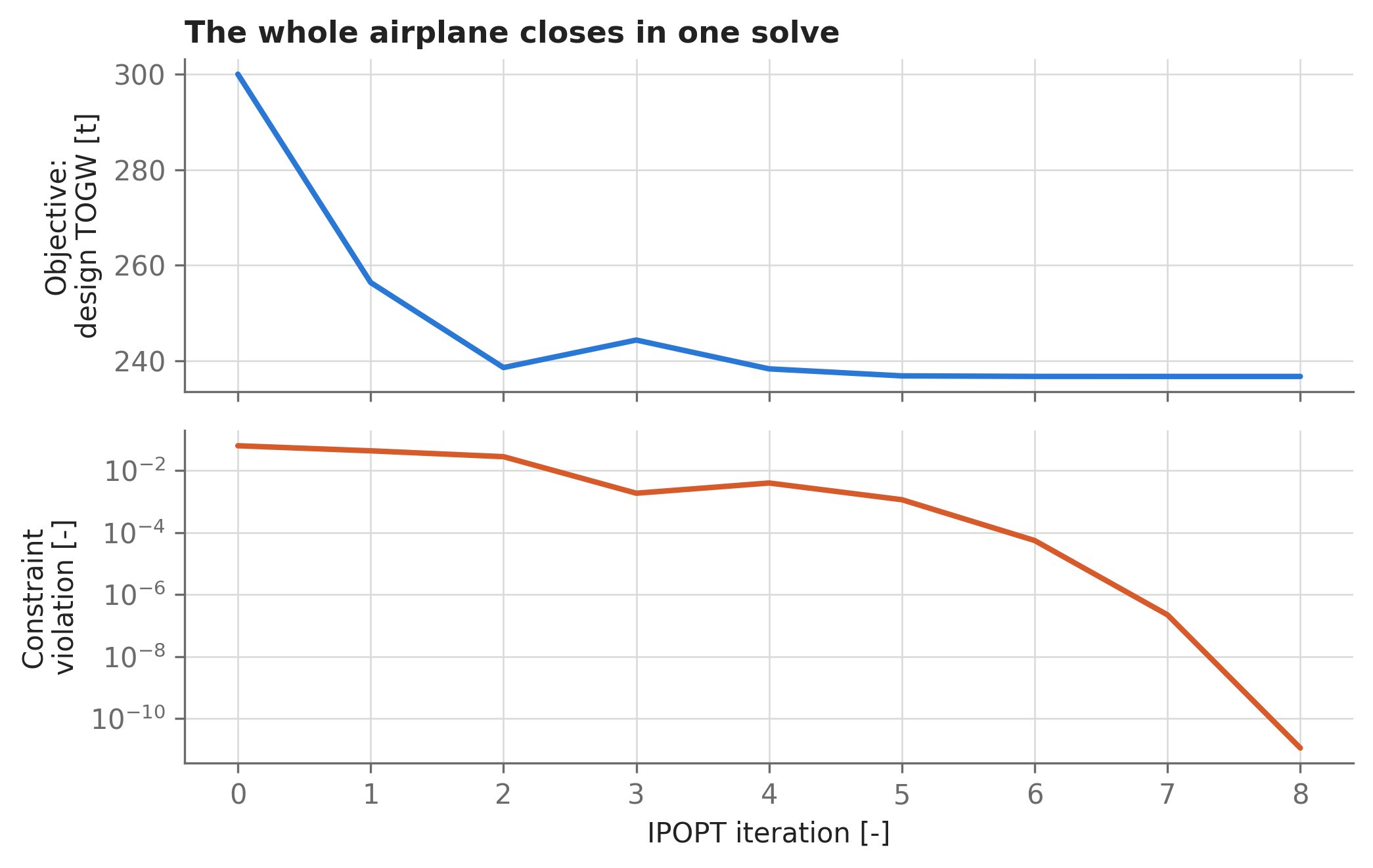
Converged: True, 8 iterations, 2.8 sThe entire airplane — aerodynamics, twenty-odd weight components, engine scaling, and mission — closes in 8 IPOPT iterations. For perspective: that is comparable to what a bare textbook sizing loop takes to converge its single weight variable, except here each iteration also carries six design degrees of freedom toward optimality.
16.8 Results: the Jet A baseline
To pull numbers out of a solution, call it like a function on any expression from the model — sol(expr) evaluates the whole upstream graph at the optimum. We wrap the outputs we care about in a helper, since we are about to generate many solutions:
def get_outputs(s, fuel_props):
    """Extract key design outputs from a solution `s`."""
    return dict(
        TOGW=s(design_mass_TOGW),
        empty=s(mass_empty),
        fuel=s(m["fuel"]),
        fuel_energy=s(m["fuel"]) * fuel_props["specific_energy"],
        span=s(wing_span),
        area=s(wing_area),
        AR=s(wing.aspect_ratio()),
        LD=s(LD_cruise),
        CL=s(aero["CL"]),
        alpha=s(alpha_cruise),
        thrust=s(design_thrust_per_engine),
        fuse_length=s(fuselage.length()),
        tank_length=s(tank_interior_length),
    )

out_jeta = get_outputs(sol, fuels["Jet A"])
First, the airplane itself:
airplane_solved, _ = make_airplane(
    sol(wing_span),
    sol(wing_yehudi_chord),
    sol(tank_interior_length),
    fuels["Jet A"]["tank_wall_thickness"],
)
three_view = airplane_solved.draw_three_view()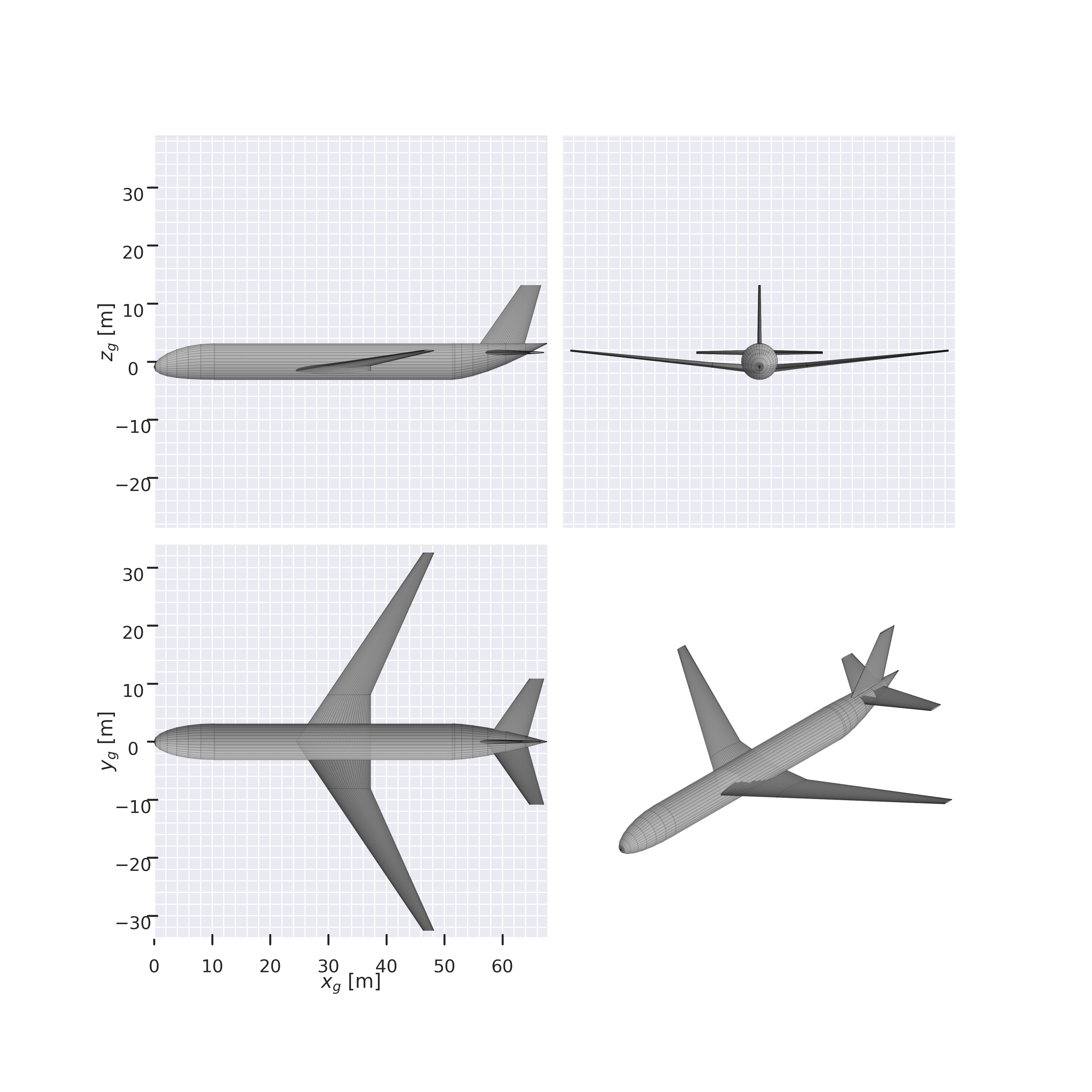
How did we do against a real airplane? The natural benchmark is the Boeing 777-300ER, whose design mission (396 passengers, 7,370 nmi, GE90 engines) nearly matches ours:
| Quantity | This model | 777-300ER |
|---|---|---|
| Wing span [m] | 65.0 | 64.8 |
| Wing aspect ratio [-] | 11.0 | 9.6 |
| Wing area [m²] | 389 | 436.8 |
| Cruise L/D [-] | 20.1 | ~19 (est.) |
| Empty mass fraction [-] | 0.48 | 0.48 |
| Fuel mass fraction [-] | 0.35 | 0.41 (capacity) |
| Max takeoff mass [t] | 237 | 351.5 |
| Empty mass [t] | 114 | 167.8 |
| Fuel mass [t] | 84 | 145.5 (capacity) |
| Fuselage length [m] | 67.6 | 73.9 |
| Thrust per engine [klbf] | 64 | 115.3 |
Read this table in two halves. The shape of the airplane is strikingly right: the span slams into the 65 m gate-limit bound exactly as Boeing’s did (and the follow-on 777-9 grew its aspect ratio to 11 by folding its wingtips — the same escape our optimizer would take if we relaxed the bound). Cruise \(C_L\) and the empty-mass fraction land on top of the reference.
The absolute masses run about a third light, and the reasons are instructive rather than embarrassing: our mission is a single still-air Breguet cruise with a flat 5% reserve (no climb, no diversion, no winds — real route planning adds 10–20% to block fuel), the drag model is a clean-sheet estimate rather than flight-test data, and the engines are sized by a single criterion (engine-out climb) where real engines also carry takeoff-field-length and time-to-climb requirements — hence the thrust gap. Lighter fuel compounds into a lighter wing, lighter gear, and so on, through exactly the same feedback loop that makes the closure converge. A conceptual model’s absolute weights are only as good as its mission definition; its trends are what we use it for, as the sweeps below show.
Post-solve sanity checks — the things a design review would ask about first:
| Check | Value | Typical long-range transport |
|---|---|---|
| Cruise \(C_L\) [-] | 0.44 | 0.4–0.55 |
| Cruise \(\alpha\) [deg] | 2.4 | 1–3 |
| Wing loading [kg/m²] | 609 | 600–800 |
| Horizontal tail volume \(V_h\) [-] | 0.98 | 0.8–1.1 |
| Vertical tail volume \(V_v\) [-] | 0.058 | 0.05–0.09 |
16.9 Switching to hydrogen
Now the payoff of parameterizing the fuel. Liquid hydrogen carries 2.8 times the energy of kerosene per kilogram — but is 12 times less dense, must live in insulated cryogenic tanks that weigh a third as much as the fuel they hold, and needs a heavier fuel system. Which effect wins? Change five parameter values and re-solve — no re-tracing, warm-started from the Jet A optimum:
opti.set_initial_from_sol(sol)

t_start = time.time()
sol_lh2 = opti.solve(
    parameter_mapping={fuel[k]: fuels["LH2"][k] for k in fuel},
    verbose=False,
)
t_lh2 = time.time() - t_start

out_lh2 = get_outputs(sol_lh2, fuels["LH2"])
print(f"Converged: {sol_lh2.stats()['success']}, "
      f"{sol_lh2.stats()['iter_count']} iterations, {t_lh2:.1f} s")
Converged: True, 23 iterations, 2.6 s| Quantity | Jet A | LH2 |
|---|---|---|
| Max takeoff mass [t] | 237 | 176 |
| Empty mass [t] | 114 | 109 |
| Fuel mass [t] | 83.6 | 28.2 |
| Fuel energy [GJ] | 3597 | 3384 |
| Tank interior length (each) [m] | 1.7 | 6.9 |
| Fuselage length [m] | 67.6 | 78.3 |
| Wing span [m] | 65.0 | 58.9 |
| Cruise L/D [-] | 20.1 | 17.9 |
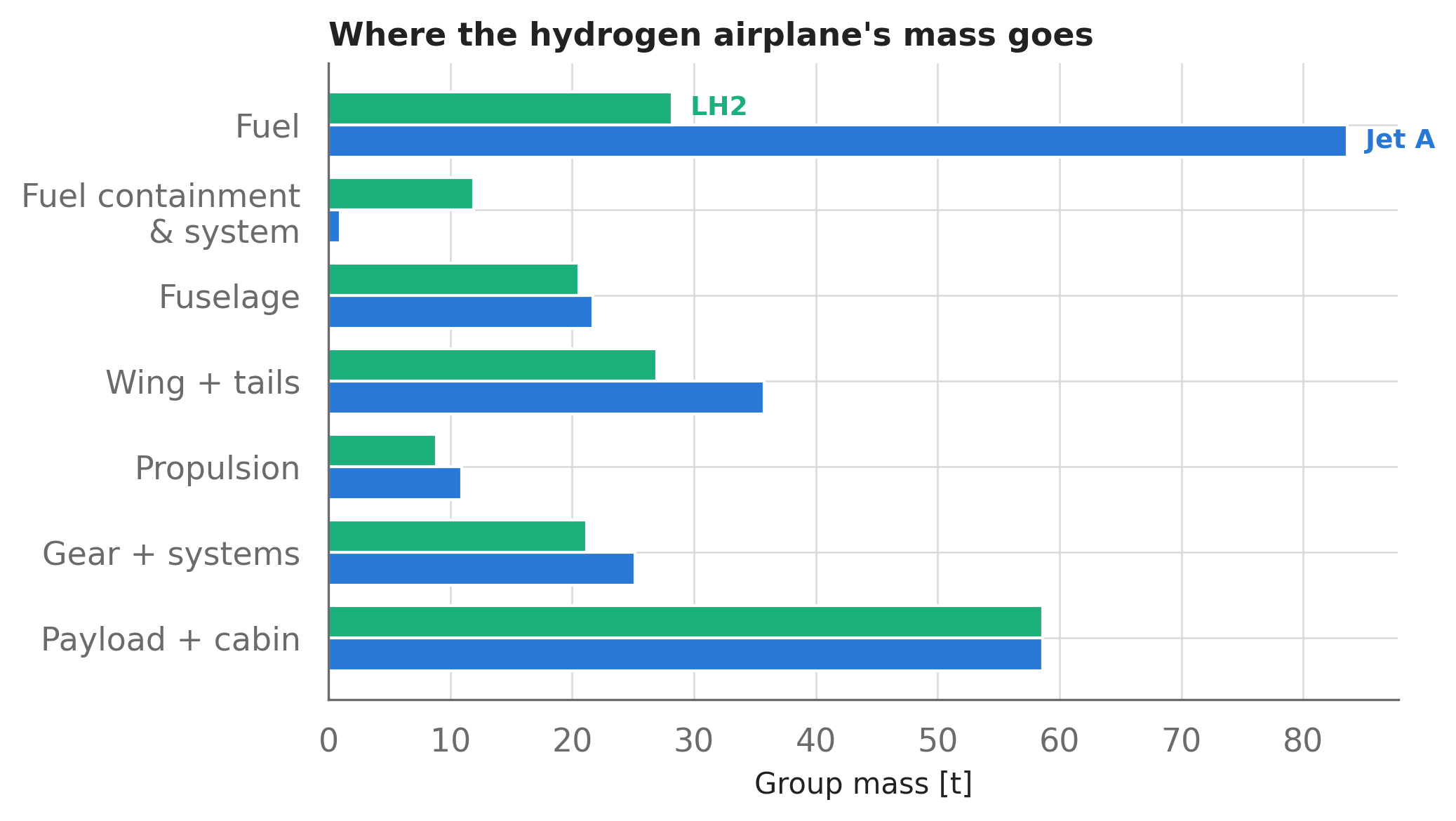
The verdict at this design range: the hydrogen airplane takes off 26% lighter — kerosene’s fuel mass simply dwarfs hydrogen’s — and carries 6% less onboard energy. The catch is visible in the geometry: the fuselage stretches by 11 m to swallow the cryogenic tanks, and the tankage-plus-fuel-system group grows several-fold, clawing back part of the energy win as drag and structure. (Whether the trade is good also depends on how the hydrogen is made — a question outside this model’s boundary.)
16.10 Tradeoff sweeps
With parameters in place, sweeping the design space is a for loop. Each solve is warm-started from its neighbor, so the whole sweep costs less than a handful of cold solves.
sweep_ranges = np.array([3000, 4500, 6000, 7500, 8500]) * u.naut_mile

sweep = {}
for fuel_name in fuels:
    outs = []
    opti.set_initial_from_sol(sol)  # restart each fuel's sweep from the baseline
    for R in sweep_ranges:
        sol_i = opti.solve(
            parameter_mapping={
                mission_range: R,
                **{fuel[k]: fuels[fuel_name][k] for k in fuel},
            },
            verbose=False,
        )
        opti.set_initial_from_sol(sol_i)  # warm-start the next point
        outs.append(get_outputs(sol_i, fuels[fuel_name]))
    sweep[fuel_name] = outs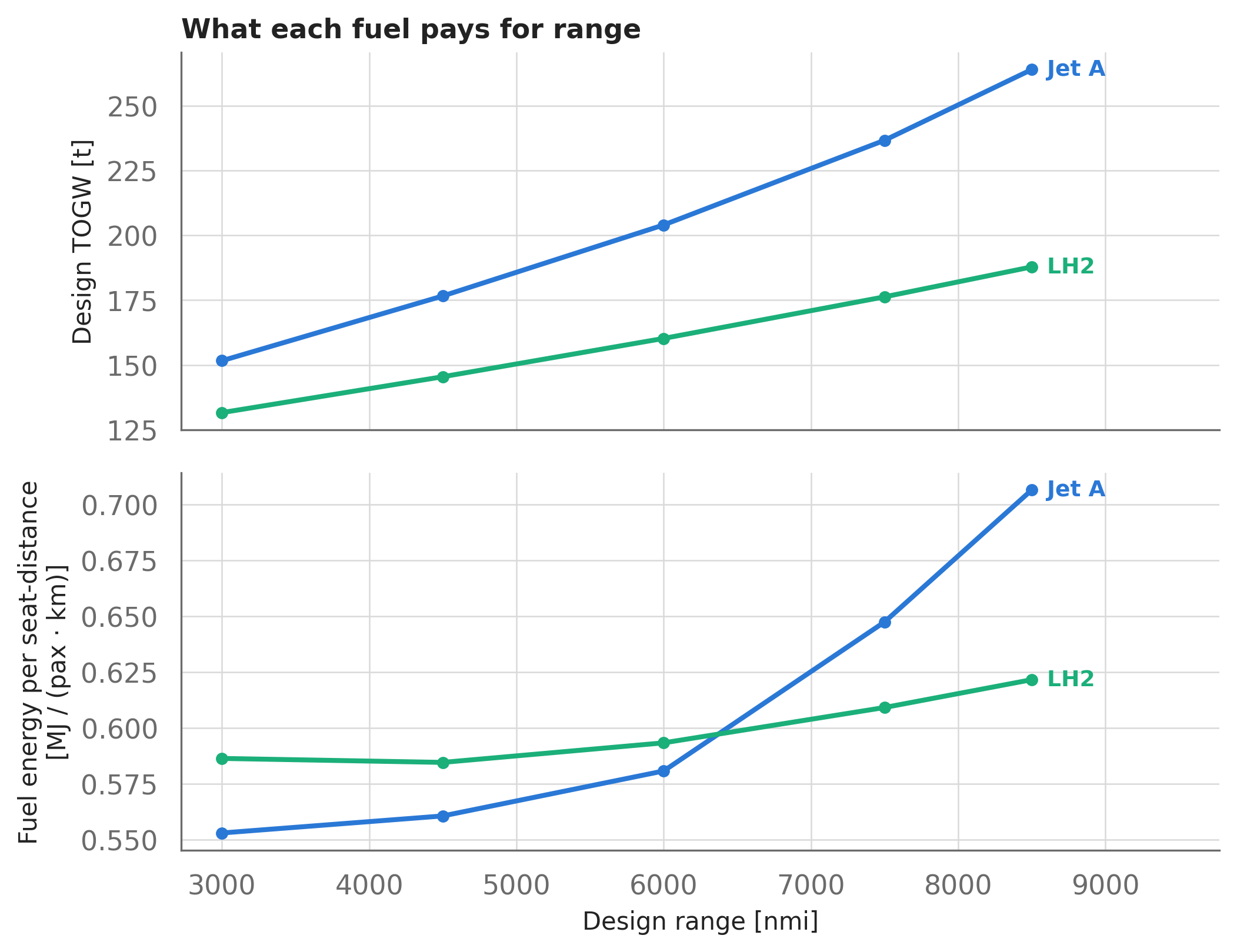
The physics behind the crossing trends: kerosene fuel mass compounds — fuel burned early in cruise must itself be lifted and dragged for hours first, so TOGW grows super-linearly with design range. Hydrogen’s fuel mass is small enough that this compounding barely bites; its penalty is instead a fixed-rate tax of tank mass and fuselage stretch per unit fuel volume. A compounding cost versus a linear one: hydrogen’s case strengthens as the design range grows, which is exactly Brewer’s classic 1970s result recovered by a model you can read in one sitting.
16.11 What we simplified
An honest accounting of what this deliberately compact model freezes or omits, roughly in order of how much each would matter for a real study:
- No pitch trim or stability closure. We check tail volumes post-solve but do not compute a CG envelope or trim the elevator; the tails are frozen at 777-scale. The source study (
lh2_airplane.py) carries fullMassProperties(CG + inertia) per component for exactly this purpose. - Wing sweep, cruise Mach, and altitude are frozen. The sweep/thickness/Mach transonic trade needs finer-grained wave-drag and structural models before an optimizer can be trusted to explore it.
- Point-mass cruise, Breguet mission. No climb, descent, or step-cruise; reserves are a flat 5% of fuel rather than a diversion-mission calculation.
- Rubber-engine propulsion. TSFC is constant with altitude and throttle; no thrust-lapse model (cruise thrust is checked implicitly through the engine-out sizing, which dominates for a twin).
- Fuselage fuel tanks for both fuels. Physically right for LH2, conservative for Jet A (real kerosene transports use integral wing tanks).
Each of these is an extension, not a rewrite: every one couples into the same opti object through shared variables, which is the whole argument for building design models this way.
16.12 Where to go next
- The aerostructural wing design study shows the same philosophy applied deep rather than wide: two disciplines coupled tightly through shared optimization variables.
- The SimPleAC chapter is this chapter’s minimal sibling — the same closure logic in ~30 lines, small enough to reason about analytically.
- The solar UAV design study swaps the mission energy source entirely: energy closure over a day-night cycle instead of a fuel tank.