import aerosandbox as asb
import aerosandbox.numpy as np
from types import SimpleNamespace


def make_cruise_problem() -> SimpleNamespace:
    """Minimum-power steady level flight of a small electric airplane."""
    opti = asb.Opti()

    ### Fixed design data
    AR = 8.0  # wing aspect ratio [-]
    e = 0.90  # Oswald span efficiency factor [-]

    ### Parameters: model inputs we may want to sweep or perturb later
    W = opti.parameter(value=8000)  # aircraft weight [N]
    CD0 = opti.parameter(value=0.030)  # zero-lift drag coefficient [-]
    CL_max = opti.parameter(value=1.6)  # maximum usable lift coefficient [-]
    rho = opti.parameter(value=1.225)  # air density [kg/m^3]
    S = opti.parameter(value=10.0)  # wing reference area [m^2]

    ### Design variables
    V = opti.variable(init_guess=30, scale=10)  # true airspeed [m/s]
    CL = opti.variable(init_guess=1.0)  # cruise lift coefficient [-]

    ### Physics
    q = 0.5 * rho * V**2  # dynamic pressure [Pa]
    CD = CD0 + CL**2 / (np.pi * AR * e)  # parabolic drag polar [-]
    D = q * S * CD  # drag [N]
    P = D * V  # power required [W]

    ### Constraints. Note: `subject_to` returns the dual variable of each constraint.
    lift_dual = opti.subject_to(q * S * CL == W)  # lift equals weight
    stall_dual = opti.subject_to(CL <= CL_max)  # stall margin

    opti.minimize(P)

return SimpleNamespace(**locals()) # bundle every local into one handle4 Solvers and Solutions
5 Solvers and Solutions
This chapter is about everything that happens after you write opti.solve() — and everything you can get back out. You will learn how to read IPOPT’s iteration log and exit codes, how to control the solver (iteration limits, callbacks, raw IPOPT options), how to extract sensitivities from a converged solution (shadow prices of constraints, and the derivative of the optimum with respect to every input parameter — for free, with no extra solves), how to run design sweeps efficiently with warm starts, how to pose feasibility problems that have no objective at all, and how to debug a solve that fails. These are the skills that turn a single optimization answer into engineering understanding: a converged solution is not just a point — it is a point plus a full set of local derivatives of your design space.
5.1 A running example: minimum-power cruise
Throughout this chapter we use one small, physical problem: an airplane in steady, level flight, trimmed to fly at whatever speed minimizes the electrical power it draws. Fly too fast and parasite drag (\(\propto V^3\) in power) eats you alive; fly too slow and you must operate at high lift coefficient, where induced drag dominates — and eventually you stall. Somewhere in between is the minimum-power speed, which is what an electric aircraft flies at to maximize endurance.
Two modeling choices below matter for the rest of the chapter:
- Inputs we may want to vary later — weight, air density, drag level — are declared with
opti.parameter()rather than hard-coded as Python floats. A parameter is a symbolic constant: the solver never optimizes it, but you can change its value between solves without rebuilding the problem, and you can ask for the sensitivity of the optimum with respect to it. opti.subject_to()returns the dual variable of each constraint, and we save those return values. We’ll cash them in later in Section 5.4.
We also wrap the whole problem in a function. This costs three lines and pays for itself immediately: every section of this chapter can create a fresh, untouched copy of the problem whenever it needs one.
Solving it takes a few milliseconds:
prob = make_cruise_problem()
sol = prob.opti.solve(verbose=False)

print(f"V*  = {sol(prob.V):7.2f} m/s")
print(f"CL* = {sol(prob.CL):7.3f}")
print(f"P*  = {sol(prob.P) / 1e3:7.2f} kW")
V* = 30.26 m/s
CL* = 1.427
P* = 20.36 kWFigure 5.1 shows what the optimizer just did. With the lift constraint substituted in (each airspeed implies a required \(C_L\)), power required is a one-dimensional function of airspeed, and the solver has found its minimum: 20.4 kW at 30.3 m/s. Note how close the optimum sits to the stall boundary at 28.6 m/s — minimum-power flight happens uncomfortably close to stall, which is why endurance-optimized aircraft (and soaring birds) fly so slowly.
Show plotting code
import _common
import matplotlib.pyplot as plt

# Numeric values of the parameters, extracted from the solution:
W0, CD00, CL_max0, rho0, S0 = sol([prob.W, prob.CD0, prob.CL_max, prob.rho, prob.S])

V_plot = np.linspace(24, 46, 300)
q_plot = 0.5 * rho0 * V_plot**2
CL_req = W0 / (q_plot * S0)  # lift coefficient required for L = W
P_plot = q_plot * S0 * (CD00 + CL_req**2 / (np.pi * prob.AR * prob.e)) * V_plot
V_stall = np.sqrt(2 * W0 / (rho0 * S0 * CL_max0))

fig, ax = plt.subplots(figsize=(7, 4))
ax.plot(V_plot, P_plot / 1e3, color=_common.SERIES[0])
ax.axvspan(V_plot.min(), V_stall, color=_common.GRID, alpha=0.6, zorder=0)
ax.text(
    V_stall - 0.4, P_plot.max() / 1e3, "stalled:\nrequires $C_L > C_{L,\\max}$",
    ha="right", va="top", fontsize=9, color=_common.TEXT_SECONDARY,
)
ax.set_xlim(V_plot.min(), V_plot.max())
ax.plot(sol(prob.V), sol(prob.P) / 1e3, "o", color=_common.SERIES[3], zorder=5)
ax.annotate(
    "optimum",
    xy=(sol(prob.V), sol(prob.P) / 1e3),
    xytext=(sol(prob.V) + 1.2, sol(prob.P) / 1e3 + 0.4),
    color=_common.SERIES[3], fontweight="bold", fontsize=9, va="bottom",
)
ax.set_xlabel("Airspeed $V$ [m/s]")
ax.set_ylabel("Power required [kW]")
ax.set_title("Minimum-power cruise: the design space the solver searches")
plt.show()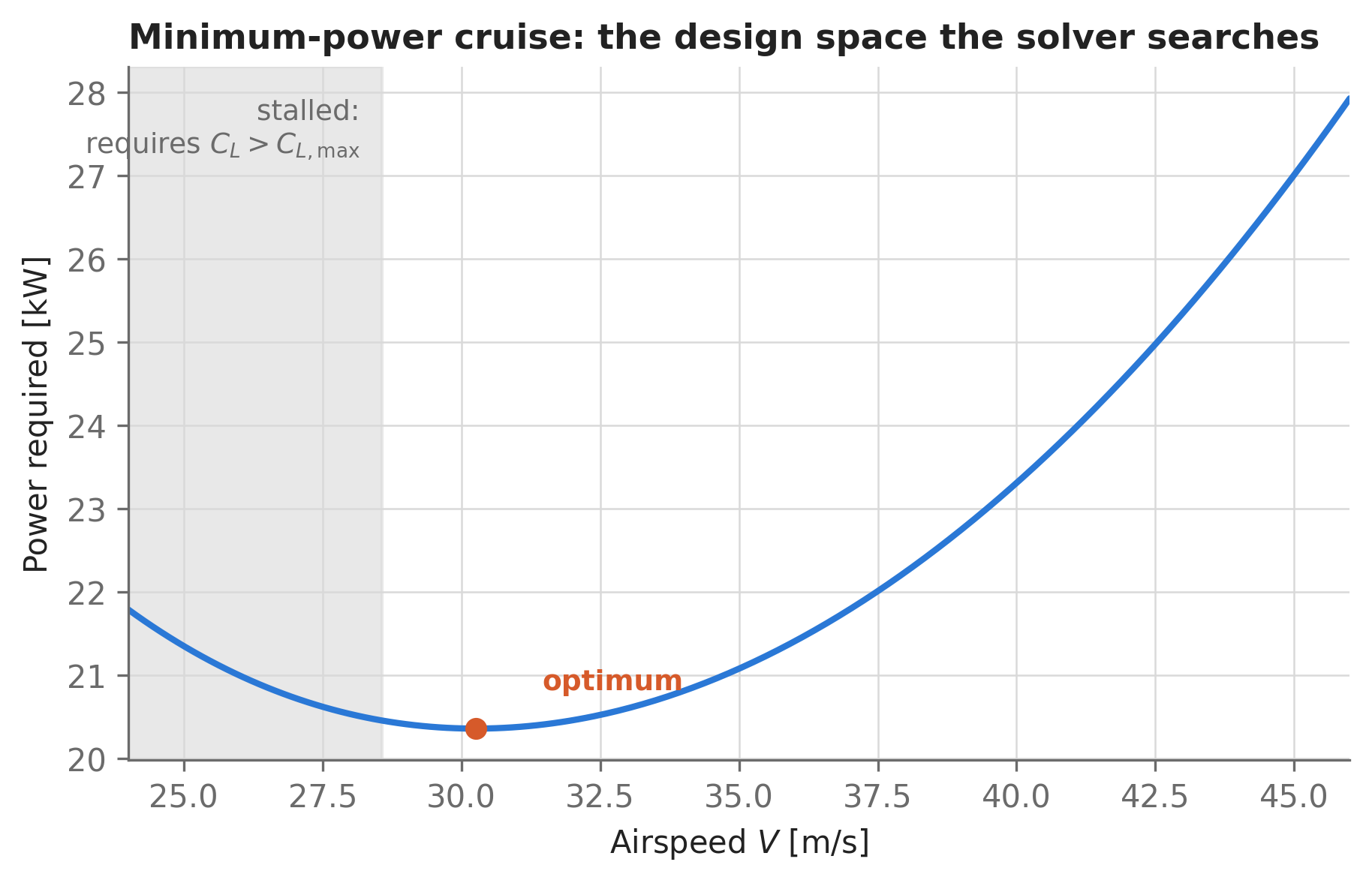
5.2 Reading the solver’s output
By default (verbose=True), opti.solve() streams IPOPT’s progress to the console. Here is the same solve again, this time with the log visible:
sol = prob.opti.solve()This is Ipopt version 3.14.11, running with linear solver MUMPS 5.4.1.
Number of nonzeros in equality constraint Jacobian...: 2
Number of nonzeros in inequality constraint Jacobian.: 1
Number of nonzeros in Lagrangian Hessian.............: 3
Total number of variables............................: 2
variables with only lower bounds: 0
variables with lower and upper bounds: 0
variables with only upper bounds: 0
Total number of equality constraints.................: 1
Total number of inequality constraints...............: 1
inequality constraints with only lower bounds: 0
inequality constraints with lower and upper bounds: 0
inequality constraints with only upper bounds: 1
iter objective inf_pr inf_du lg(mu) ||d|| lg(rg) alpha_du alpha_pr ls
0 1.2272430e+04 2.49e+03 8.79e+00 0.0 0.00e+00 - 0.00e+00 0.00e+00 0
1 2.0654046e+04 7.75e+01 1.11e+00 -6.2 4.19e-01 - 1.00e+00 1.00e+00h 1
2 2.0356513e+04 1.98e-01 6.24e-04 -6.9 2.29e-02 - 1.00e+00 1.00e+00f 1
3 2.0357266e+04 8.77e-04 5.65e-05 -8.3 5.58e-04 - 9.98e-01 1.00e+00h 1
4 2.0357269e+04 1.44e-08 6.42e-09 -10.6 2.26e-06 - 1.00e+00 1.00e+00h 1
Number of Iterations....: 4
(scaled) (unscaled)
Objective...............: 1.3922013076967218e+02 2.0357269265714564e+04
Dual infeasibility......: 6.4207017108674005e-09 9.3885814415163141e-07
Constraint violation....: 2.6089505159429144e-10 1.4381839719135316e-08
Variable bound violation: 0.0000000000000000e+00 0.0000000000000000e+00
Complementarity.........: 1.4805852913290367e-09 2.1649651727670632e-07
Overall NLP error.......: 6.4207017108674005e-09 9.3885814415163141e-07
Number of objective function evaluations = 5
Number of objective gradient evaluations = 5
Number of equality constraint evaluations = 5
Number of inequality constraint evaluations = 5
Number of equality constraint Jacobian evaluations = 5
Number of inequality constraint Jacobian evaluations = 5
Number of Lagrangian Hessian evaluations = 4
Total seconds in IPOPT = 0.003
EXIT: Optimal Solution Found.
solver : t_proc (avg) t_wall (avg) n_eval
nlp_f | 20.00us ( 4.00us) 16.72us ( 3.34us) 5
nlp_g | 25.00us ( 5.00us) 19.84us ( 3.97us) 5
nlp_grad_f | 40.00us ( 6.67us) 32.24us ( 5.37us) 6
nlp_hess_l | 30.00us ( 7.50us) 28.23us ( 7.06us) 4
nlp_jac_g | 26.00us ( 4.33us) 27.73us ( 4.62us) 6
total | 3.70ms ( 3.70ms) 3.52ms ( 3.52ms) 1The preamble counts variables and constraints (here 2 variables, 2 constraints) and reports the sparsity of the constraint Jacobian and Lagrangian Hessian — for large problems, sparsity is what keeps solves fast. Then comes the iteration table. The columns you’ll actually use:
| Column | Meaning |
|---|---|
objective |
Current value of the objective function. |
inf_pr |
Primal infeasibility: the worst constraint violation. Must go to ~0 for a valid solution. |
inf_du |
Dual infeasibility: how far the point is from satisfying the local optimality (KKT) conditions. |
lg(mu) |
\(\log_{10}\) of the interior-point barrier parameter; drifts toward \(-9\) or so as the solver homes in. |
||d|| |
Size of the step just taken in the (scaled) variable space. |
lg(rg) |
\(\log_{10}\) of Hessian regularization; - means none was needed (good — the problem looks locally convex). |
alpha_pr, alpha_du |
Fraction of the full step accepted for primal/dual variables. Persistent tiny values signal trouble (usually scaling — see the previous chapter). |
ls |
Number of line-search trials; 1 is ideal. |
A healthy solve looks exactly like the one above: inf_pr and inf_du plummet super-linearly over the last few iterations (a hallmark of Newton’s method near a solution), step acceptance alpha_pr approaches 1, and the log ends with EXIT: Optimal Solution Found.
The same information is available programmatically through sol.stats():
stats = sol.stats()
print("success:       ", stats["success"])
print("return_status: ", stats["return_status"])
print("iterations:    ", stats["iter_count"])
success: True
return_status: Solve_Succeeded
iterations: 4(stats["iterations"] additionally holds the full per-iteration history — obj, inf_pr, inf_du, and so on as arrays — which is handy for plotting convergence without re-running anything.)
The return_status values you are most likely to meet:
return_status |
What it means |
|---|---|
Solve_Succeeded |
Converged to the requested tolerance. |
Solved_To_Acceptable_Level |
Converged, but only to the looser “acceptable” tolerance. Usually fine; often a scaling smell. |
Infeasible_Problem_Detected |
IPOPT is locally convinced no feasible point exists. See Section 5.7. |
Maximum_Iterations_Exceeded |
Ran out of iterations (max_iter). |
Maximum_CpuTime_Exceeded |
Ran out of wall time (max_runtime). |
Restoration_Failed |
The feasibility-restoration phase itself failed — frequently a symptom of NaNs or terrible scaling. |
Invalid_Number_Detected |
A NaN/Inf appeared in a function or derivative. See the previous chapter for NaN-proofing. |
5.3 Controlling the solver
All solver control flows through keyword arguments of opti.solve(). The ones you’ll use routinely (all verified against the current API):
| Argument | Default | Purpose |
|---|---|---|
verbose |
True |
Set False to silence IPOPT entirely — essential inside sweeps. |
max_iter |
1000 |
Iteration budget. IPOPT scales superbly, so hitting 1000 usually means a modeling problem, not a hard problem. |
max_runtime |
1e20 |
Wall-clock budget in seconds (maps to ipopt.max_cpu_time). |
parameter_mapping |
None |
{parameter: value} dict to re-point parameters before solving — the engine behind sweeps (Section 5.5). |
callback |
None |
A func(iteration_number) called at every iteration. |
behavior_on_failure |
"raise" |
"return_last" returns the last iterate (with a warning) instead of raising — invaluable for sweeps and debugging. |
options |
None |
Raw option dict passed straight to CasADi/IPOPT for anything not covered above. |
For example, capping iterations — useful to bail out early on hopeless points during a sweep:
sol_capped = prob.opti.solve(
    max_iter=3, verbose=False, behavior_on_failure="return_last"
)
print(sol_capped.stats()["return_status"])Maximum_Iterations_Exceeded/home/psharpe/gh/AeroSandbox/aerosandbox/optimization/opti.py:845: UserWarning: Optimization failed. Returning last solution.
warnings.warn("Optimization failed. Returning last solution.")And passing a raw IPOPT option (the full catalog is in the IPOPT options reference) — here, a tighter convergence tolerance:
sol_tight = prob.opti.solve(options={"ipopt.tol": 1e-12}, verbose=False)
print(f"{sol_tight.stats()['iter_count']} iterations to tol = 1e-12")
5 iterations to tol = 1e-125.3.1 Watching a solve with callbacks
A callback is a function invoked at every iteration. Inside it, opti.debug.value(expression) evaluates any expression at the solver’s current iterate — mid-solve, before any solution exists. This is the standard way to record the path the optimizer takes.
Here we restart the cruise problem from a deliberately terrible initial guess (100 m/s — over three times the optimal speed) and log both the objective and the lift-constraint violation at every iteration. Note opti.set_initial(), which overrides a variable’s initial guess after the problem is built — we will meet it again as the warm-start mechanism in Section 5.5.
prob2 = make_cruise_problem()
prob2.opti.set_initial(prob2.V, 100)  # a deliberately bad starting point
prob2.opti.set_initial(prob2.CL, 0.3)

history = []


def log_progress(iteration_number: int) -> None:
    history.append(
        dict(
            P=prob2.opti.debug.value(prob2.P),
            lift_error=abs(prob2.opti.debug.value(prob2.q * prob2.S * prob2.CL - prob2.W)),
        )
    )


sol2 = prob2.opti.solve(callback=log_progress, verbose=False)
print(f"Converged in {len(history)} iterations, from a guess 3.3x too fast.")
Converged in 8 iterations, from a guess 3.3x too fast.Show plotting code
import _common

iters = np.arange(len(history))
P_hist = np.array([h["P"] for h in history])
err_hist = np.array([h["lift_error"] for h in history])

fig, axs = plt.subplots(2, 1, figsize=(7, 5.5), sharex=True)
axs[0].plot(iters, P_hist / 1e3, ".-", color=_common.SERIES[0])
axs[0].axhline(sol2(prob2.P) / 1e3, color=_common.GRID, zorder=0)
axs[0].set_ylabel("Objective: power $P$ [kW]")
axs[0].set_title("What IPOPT was thinking, iteration by iteration")
axs[1].semilogy(iters, np.maximum(err_hist, 1e-16), ".-", color=_common.SERIES[1])
axs[1].set_ylabel("Lift constraint violation [N]")
axs[1].set_xlabel("IPOPT iteration [-]")
plt.show()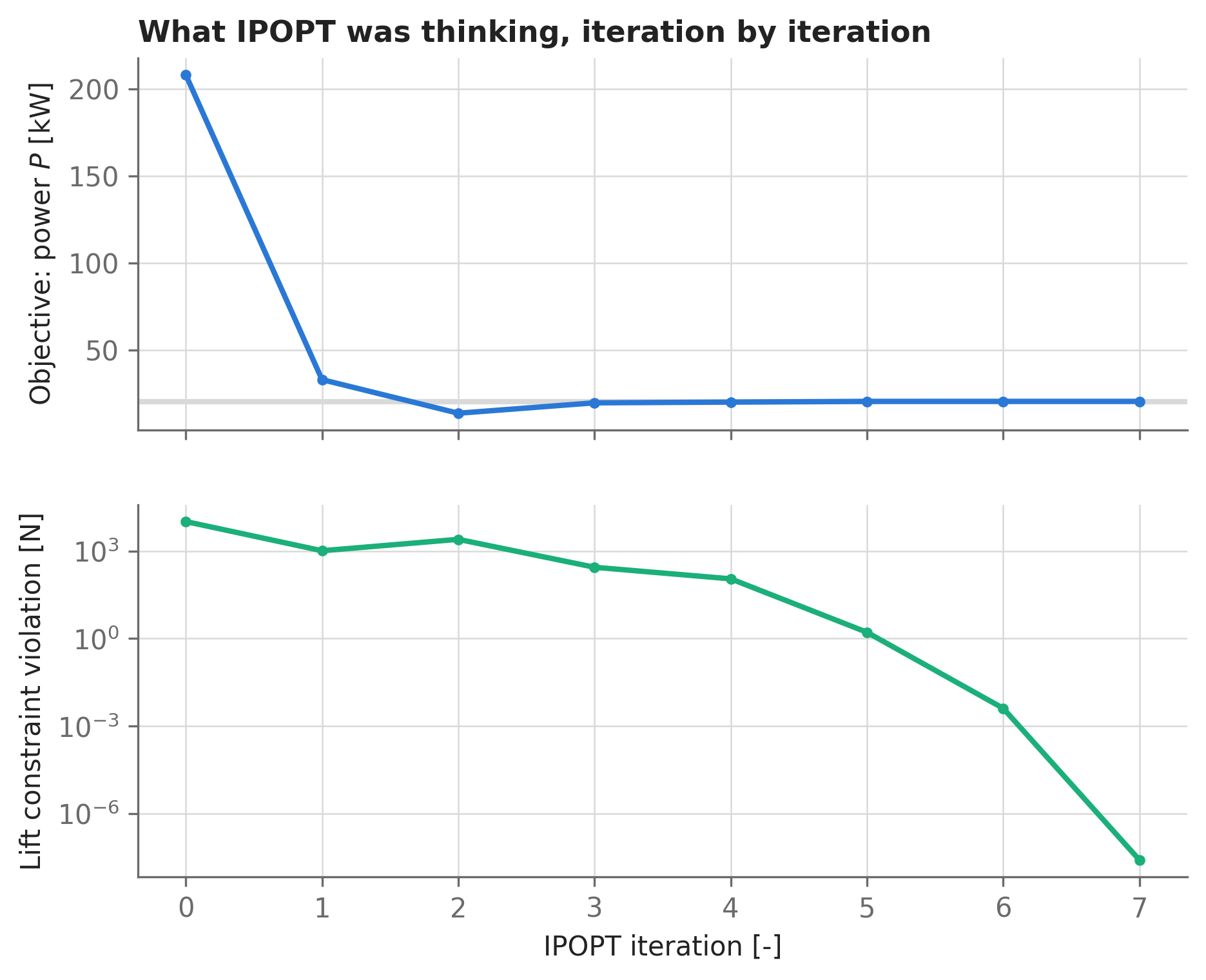
5.4 Solutions carry sensitivities
A converged interior-point solution contains more than optimal variable values: it also contains the dual variables (Lagrange multipliers) of every constraint. The dual of a constraint is its shadow price — the rate at which the optimal objective would change if you relaxed or tightened that constraint by one unit. In design terms: shadow prices are the exchange rates of your requirements.
In AeroSandbox, opti.subject_to() returns the dual variable directly; evaluate it through the solution like any other quantity. We saved both duals when we built the problem:
sol = prob.opti.solve(verbose=False)  # re-solve at nominal parameters

print(f"Shadow price of weight:       {sol(prob.lift_dual):.3f} W per N")
print(f"Shadow price of stall margin: {sol(prob.stall_dual):.1e} W per unit CL_max")
Shadow price of weight: 3.817 W per N
Shadow price of stall margin: 3.1e-07 W per unit CL_maxTwo lessons here. First, the lift constraint’s dual says each newton of extra weight costs 3.82 W of cruise power — about 37 W per kilogram. Before you’ve run a single trade study, the solution has already priced weight growth for you. (Sanity check: multiplying the dual by \(W/P^*\) gives 1.5000 — exactly \(3/2\), as it must, since minimum power scales as \(W^{3/2}\). More on that scaling in a moment.)
Second, the stall constraint’s dual is zero to solver precision. That is complementary slackness: the optimizer chose \(C_L^* =\) 1.43, comfortably below \(C_{L,\max} = 1.6\), so the constraint is inactive and relaxing it is worth nothing. Watch what happens if we drop \(C_{L,\max}\) to 1.3 — now the stall limit bites, and its shadow price wakes up:
sol_lowCL = prob.opti.solve(parameter_mapping={prob.CL_max: 1.3}, verbose=False)

print(f"CL* = {sol_lowCL(prob.CL):.3f}  (pinned at CL_max)")
print(f"P*  = {sol_lowCL(prob.P) / 1e3:.2f} kW  (was {sol(prob.P) / 1e3:.2f} kW)")
print(f"Shadow price of stall margin: {sol_lowCL(prob.stall_dual):.0f} W per unit CL_max")
CL* = 1.300 (pinned at CL_max)
P* = 20.43 kW (was 20.36 kW)
Shadow price of stall margin: 1147 W per unit CL_maxThat number is a direct verdict on a design change: a flap system that added 0.1 of usable \(C_{L,\max}\) would save about 115 W of cruise power on this constrained design — weigh that against the flap’s mass (priced by the other dual!) and you have a principled trade, from one solve.
Parameter values persist on the Opti object, so before moving on we put \(C_{L,\max}\) back and re-solve at the nominal design point:
prob.opti.set_value(prob.CL_max, 1.6)  # restore the nominal value
sol = prob.opti.solve(verbose=False)
NoteSign convention
AeroSandbox (via CasADi) reports duals as nonnegative magnitudes: \(|\partial J^* / \partial(\text{constraint bound})|\). For an active inequality, the direction is never ambiguous — tightening it always hurts the objective, relaxing always helps (and inactive inequalities price at zero). For an equality, reason physically about the direction, or read the signed value from the parameter-sensitivity machinery below. One more caveat: duals are quoted in the units of your objective as written — if you opti.minimize(P / 1e3) for scaling reasons, the duals scale by the same factor.
5.4.1 The sensitivity of the optimum to every parameter, at once
Shadow prices generalize. For any parameter \(p\) (declared via opti.parameter()), the derivative of the optimal objective is given by the gradient of the Lagrangian \(\mathcal{L} = f + \lambda^\top g\), evaluated at the solution — no extra solves, no finite differencing, no re-converging. This is the same adjoint identity that makes geometric-programming sensitivity reports (à la GPKit) so prized, and it works here for arbitrary nonconvex problems. The helper below assembles the Lagrangian from quantities every solved Opti already carries (opti.f, opti.g, the bound vectors, and the multipliers opti.lam_g) and differentiates it with respect to the full parameter vector opti.p in one shot:
import casadi as cas


def solution_sensitivities(opti: asb.Opti, sol: asb.OptiSol) -> np.ndarray:
    """d(optimal objective)/d(parameter), for every parameter of `opti`.

    Evaluates the gradient of the Lagrangian w.r.t. the parameter vector at the
    solution. IPOPT's multiplier convention: lam_g > 0 means the constraint's
    upper bound is active; lam_g < 0, its lower bound.
    """
    lam = opti.lam_g
    # Infinite bounds are constants (zero parameter-gradient); zero them out
    # so they can't produce inf * 0 = NaN:
    lbg = cas.if_else(opti.lbg > -1e15, opti.lbg, 0)
    ubg = cas.if_else(opti.ubg < 1e15, opti.ubg, 0)
    lagrangian = (
        opti.f
        + cas.dot(cas.fmax(lam, 0), opti.g - ubg)
        + cas.dot(cas.fmin(lam, 0), opti.g - lbg)
    )
    return sol.value(cas.gradient(lagrangian, opti.p))
Before trusting it, let’s give ourselves something exact to check against. Eliminating the lift constraint analytically (\(V = \sqrt{2W / (\rho S C_L)}\)) turns cruise power into
\[ P = W^{3/2} \sqrt{\frac{2}{\rho S}} \; \frac{C_D}{C_L^{3/2}}, \]
and since the optimal \(C_L\) depends only on the drag polar (at the minimum, induced drag is exactly three times parasite drag, so \(C_D^* = 4\,C_{D_0}\)), the optimum obeys a clean power law: \(P^* \propto W^{3/2}\, \rho^{-1/2}\, S^{-1/2}\, C_{D_0}^{1/4}\). So the log-log sensitivities \(\frac{p}{J^*}\frac{\partial J^*}{\partial p}\) — “percent change in optimal power per percent change in input” — should come out to exactly \(1.5\), \(-0.5\), \(-0.5\), and \(0.25\), with \(C_{L,\max}\) (inactive) at zero. Here’s the test, with brute-force central finite differences (two extra solves per parameter) alongside:
names = ["W [N]", "CD0 [-]", "CL_max [-]", "rho [kg/m^3]", "S [m^2]"]
params = [prob.W, prob.CD0, prob.CL_max, prob.rho, prob.S]
values = np.array(sol(params))

dP_dp = solution_sensitivities(prob.opti, sol)  # adjoint: free

dP_dp_fd = []  # finite differences: 2 solves per parameter
for param, value in zip(params, values):
    h = 1e-4 * value
    P_plus = prob.opti.solve(parameter_mapping={param: value + h}, verbose=False)(prob.P)
    P_minus = prob.opti.solve(parameter_mapping={param: value - h}, verbose=False)(prob.P)
    prob.opti.set_value(param, value)  # restore the nominal value
    dP_dp_fd.append((P_plus - P_minus) / (2 * h))
Show table-formatting code
import pandas as pd

pd.DataFrame(
    {
        "Value": [f"{v:.4g}" for v in values],
        "dP*/dp, adjoint [W/unit]": [f"{s:.4g}" for s in dP_dp],
        "dP*/dp, finite diff. [W/unit]": [f"{s:.4g}" for s in dP_dp_fd],
        "Log-log sensitivity [-]": [f"{s:.4f}" for s in dP_dp * values / sol(prob.P)],
        "Analytic exponent [-]": ["1.5", "0.25", "0", "-0.5", "-0.5"],
    },
    index=names,
)| Value | dP*/dp, adjoint [W/unit] | dP*/dp, finite diff. [W/unit] | Log-log sensitivity [-] | Analytic exponent [-] | |
|---|---|---|---|---|---|
| W [N] | 8000 | 3.817 | 3.817 | 1.5000 | 1.5 |
| CD0 [-] | 0.03 | 1.696e+05 | 1.696e+05 | 0.2500 | 0.25 |
| CL_max [-] | 1.6 | -3.111e-07 | 2.308e-06 | -0.0000 | 0 |
| rho [kg/m^3] | 1.225 | -8309 | -8309 | -0.5000 | -0.5 |
| S [m^2] | 10 | -1018 | -1018 | -0.5000 | -0.5 |
The adjoint values match finite differences to five-plus digits and land on the analytic exponents essentially exactly — and unlike sol(dual), they are signed (note the negative sensitivities to \(\rho\) and \(S\): denser air and more wing both cut minimum power). On a problem with thousands of parameters, this table still costs one solve. Two caveats: it is valid only at a converged solution, and it is a local derivative — it knows nothing about the active set changing (e.g., the stall constraint becoming active) under large parameter excursions. You will see this machinery earn its keep on a full aircraft sizing problem in the SimPleAC chapter.
5.4.2 Reaching into the AD engine directly
The Lagrangian trick above hints at something more general: because every AeroSandbox model is built on CasADi’s automatic differentiation, you can construct derivatives of your own functions and use them anywhere — including inside constraints. The classic use case is a stability requirement like \(\partial C_m / \partial \alpha < 0\), a constraint on a derivative of your model. The pattern: differentiate through a dummy symbol, wrap the result in a cas.Function, and apply it to your optimization variables.
A minimal example — find \(x\) such that \(\mathrm{d}(x^4)/\mathrm{d}x = 1\) (analytically, \(x = (1/4)^{1/3}\)):
opti = asb.Opti()
x = opti.variable(init_guess=10)


def f(x):
    return x**4


s = cas.MX.sym("s")  # dummy symbol to differentiate through
dfdx = cas.Function("dfdx", [s], [cas.gradient(f(s), s)])

opti.subject_to(dfdx(x) == 1)
sol_grad = opti.solve(verbose=False)

print(f"x = {sol_grad(x):.6f}   (analytic: {(1 / 4) ** (1 / 3):.6f})")
x = 0.629961 (analytic: 0.629961)(Notice there is no opti.minimize() here — this is our first feasibility problem, the subject of Section 5.6.)
5.5 Design sweeps
One optimum is a data point; a family of optima is a design study. Because parameters can be re-pointed without rebuilding the problem, sweeping is just re-solving in a loop with parameter_mapping:
W_range = np.linspace(5000, 12000, 15)  # aircraft weight [N]

P_opt, V_opt = [], []
for W_val in W_range:
    sol_i = prob.opti.solve(parameter_mapping={prob.W: W_val}, verbose=False)
    P_opt.append(sol_i(prob.P))
    V_opt.append(sol_i(prob.V))
P_opt, V_opt = np.array(P_opt), np.array(V_opt)

prob.opti.set_value(prob.W, sol(prob.W))  # restore the nominal weight
Figure 5.3 shows the result, along with a line we already own: the tangent predicted by the shadow price of weight from Section 5.4. The dual is the exact local slope of this sweep — the sweep and the sensitivity are two views of the same object. The tangent is an excellent approximation near the nominal point and increasingly optimistic far below it, because \(P^* \propto W^{3/2}\) curves upward; that curvature (and any active-set change) is what a dual can’t see and a sweep can.
Show plotting code
import _common

fig, axs = plt.subplots(2, 1, figsize=(7, 6), sharex=True)

axs[0].plot(W_range, P_opt / 1e3, ".-", color=_common.SERIES[0])
P_tangent = sol(prob.P) + sol(prob.lift_dual) * (W_range - sol(prob.W))
axs[0].plot(W_range, P_tangent / 1e3, "--", color=_common.SERIES[3], linewidth=1.5)
axs[0].plot(sol(prob.W), sol(prob.P) / 1e3, "o", color=_common.SERIES[3], zorder=5)
_common.label_line(
    axs[0], W_range[-1], P_opt[-1] / 1e3, "sweep of\noptima",
    color=_common.SERIES[0], dx=150, dy=0.4,
)
_common.label_line(
    axs[0], W_range[-1], P_tangent[-1] / 1e3, "tangent from\nshadow price",
    color=_common.SERIES[3], dx=150, dy=-2.2,
)
axs[0].set_xlim(right=W_range[-1] + 1900)
axs[0].set_ylabel("Optimal cruise power [kW]")
axs[0].set_title("The dual is the local slope of the sweep")

axs[1].plot(W_range, V_opt, ".-", color=_common.SERIES[1])
axs[1].set_ylabel("Optimal airspeed [m/s]")
axs[1].set_xlabel("Aircraft weight $W$ [N]")
plt.show()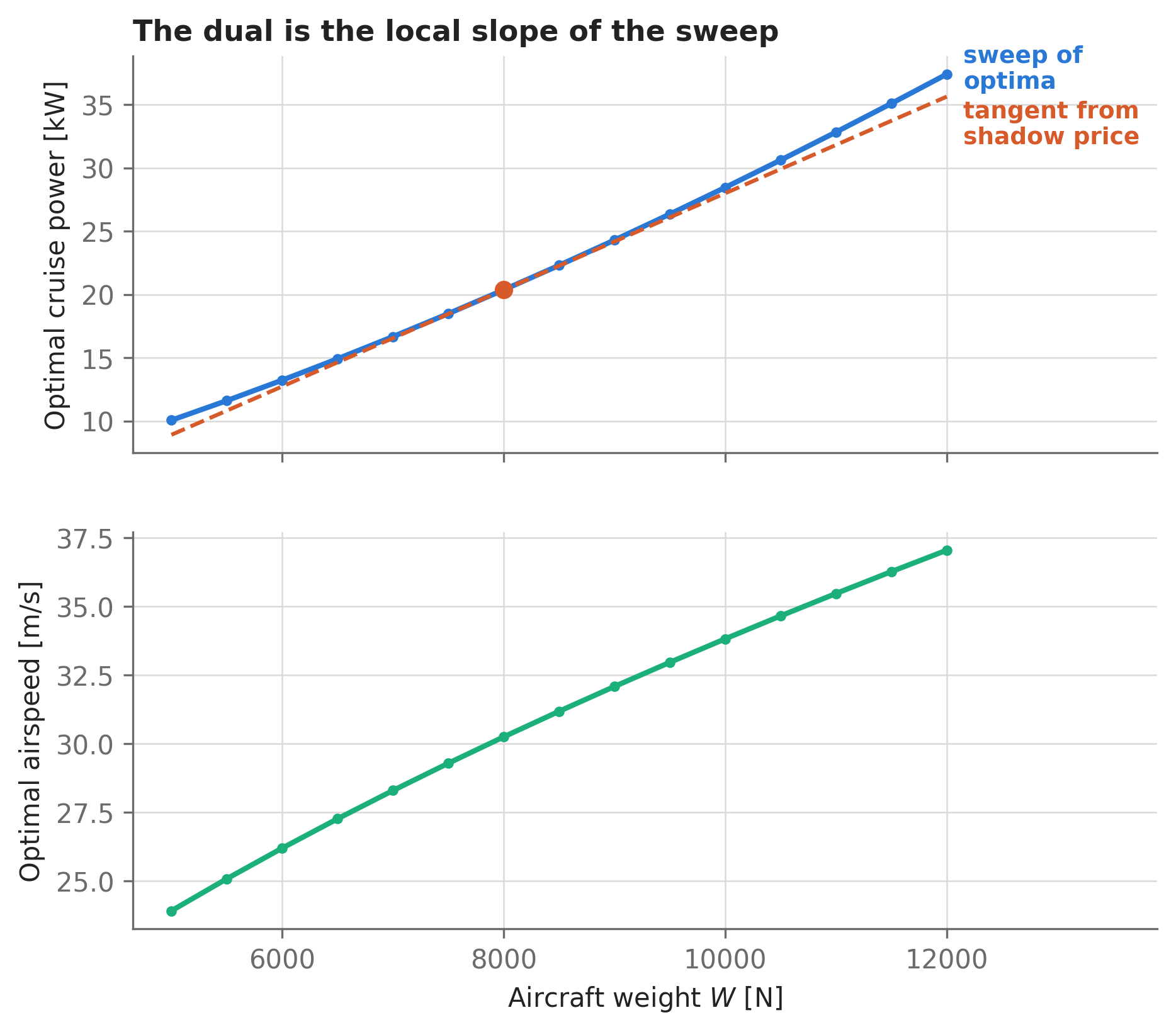
5.5.1 solve_sweep(): sweeps as a one-liner
The loop above is common enough that Opti provides it built-in. opti.solve_sweep() takes a {parameter: array_of_values} mapping, solves once per value, and returns a NumPy object-array of solutions (with None at any point where the solver failed, rather than crashing your whole study — each inner solve runs with sensible sweep defaults of verbose=False, max_iter=200, overridable via solve_kwargs):
prob = make_cruise_problem()  # fresh instance: no leftover state

sols = prob.opti.solve_sweep(parameter_mapping={prob.W: W_range})
Running optimization sweep in serial...
Run 1/15 | 5000| Solved in 6 iterations, 0.01 sec.
Run 2/15 | 5500| Solved in 5 iterations, 0.01 sec.
Run 3/15 | 6000| Solved in 5 iterations, 0.01 sec.
Run 4/15 | 6500| Solved in 5 iterations, 0.01 sec.
Run 5/15 | 7000| Solved in 5 iterations, 0.01 sec.
Run 6/15 | 7500| Solved in 5 iterations, 0.01 sec.
Run 7/15 | 8000| Solved in 4 iterations, 0.01 sec.
Run 8/15 | 8500| Solved in 4 iterations, 0.01 sec.
Run 9/15 | 9000| Solved in 5 iterations, 0.01 sec.
Run 10/15 | 9500| Solved in 5 iterations, 0.01 sec.
Run 11/15 | 10000| Solved in 5 iterations, 0.01 sec.
Run 12/15 | 10500| Solved in 5 iterations, 0.01 sec.
Run 13/15 | 11000| Solved in 5 iterations, 0.01 sec.
Run 14/15 | 11500| Solved in 5 iterations, 0.01 sec.
Run 15/15 | 12000| Solved in 5 iterations, 0.01 sec.P_swept = np.array([s(prob.P) for s in sols])
print(f"Max |difference| vs. the manual loop: {float(np.max(np.abs(P_swept - P_opt))):.2e} W")Max |difference| vs. the manual loop: 0.00e+00 W5.5.2 Warm starts
Each solve above starts from the original initial guess, even though neighboring sweep points have nearly identical solutions. Passing update_initial_guesses_between_solves=True makes each successful solve seed the next one — primal and dual variables — via opti.set_initial_from_sol() (which you can also call manually to warm-start any solve from any compatible solution):
prob = make_cruise_problem()
sols_warm = prob.opti.solve_sweep(
    parameter_mapping={prob.W: W_range},
    update_initial_guesses_between_solves=True,
    verbose=False,
)

iters_cold = sum(s.stats()["iter_count"] for s in sols)
iters_warm = sum(s.stats()["iter_count"] for s in sols_warm)
print(f"Total IPOPT iterations, cold starts: {iters_cold}")
print(f"Total IPOPT iterations, warm starts: {iters_warm}")
Total IPOPT iterations, cold starts: 74
Total IPOPT iterations, warm starts: 51A 31% saving is nothing to write home about on a two-variable problem that solves in milliseconds — but the mechanism is identical on a 10,000-variable trajectory optimization, where continuation along a parameter can be the difference between a sweep that takes minutes and one that takes hours (or doesn’t converge at all at the extreme ends). One caution: warm-starting introduces path dependence. If your problem has multiple local optima, a warm-started sweep can ride one branch past the point where another becomes better; when in doubt, spot-check a few points with cold starts.
5.5.3 Multi-parameter sweeps (carpet plots)
solve_sweep broadcasts its value arrays against each other with standard NumPy rules, so a grid sweep is just a matter of shaping. With return_callable=True it returns a function that evaluates any expression across all solutions at once (with NaN where a solve failed) — much more convenient than an object-array when all you want is plotting fodder:
prob = make_cruise_problem()
CD0_values = np.array([0.020, 0.025, 0.030, 0.035, 0.040])

value_at = prob.opti.solve_sweep(
    parameter_mapping={
        prob.W: W_range.reshape(1, -1),  # shape (1, 15)
        prob.CD0: CD0_values.reshape(-1, 1),  # shape (5, 1)  -> grid of (5, 15)
    },
    verbose=False,
    return_callable=True,
)

P_grid = value_at(prob.P)  # any expression works here
print(f"{P_grid.size} optimization problems solved; grid shape {P_grid.shape}")
75 optimization problems solved; grid shape (5, 15)Show plotting code
import _common

cmap = _common.mpl.colormaps["Blues"]
colors = cmap(np.linspace(0.45, 0.95, len(CD0_values)))

fig, ax = plt.subplots(figsize=(7, 4.5))
for P_row, CD0_val, color in zip(P_grid, CD0_values, colors):
    ax.plot(W_range, P_row / 1e3, color=color)
    _common.label_line(
        ax, W_range[-1], P_row[-1] / 1e3, f"$C_{{D_0}}$ = {CD0_val:.3f}",
        color=color, dx=120,
    )
ax.set_xlim(right=W_range[-1] + 2400)
ax.set_xlabel("Aircraft weight $W$ [N]")
ax.set_ylabel("Optimal cruise power [kW]")
ax.set_title("Carpet sweep: weight × parasite drag")
plt.show()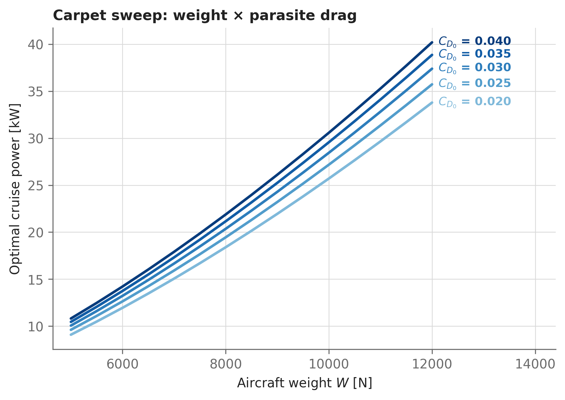
WarningSweeps mutate the
Opti object
parameter_mapping sets parameter values: after a sweep, every swept parameter keeps its last value, and with warm starts the initial guesses have moved too. That’s why the cells above rebuild with make_cruise_problem() — a fresh problem instance costs microseconds and eliminates a whole class of “why did my nominal solve change?” bugs. Wrap your problems in functions.
5.6 Feasibility problems: optimization without an objective
Sometimes you don’t want the best point — you want any point that satisfies the constraints. Skip opti.minimize() entirely (or equivalently, minimize a constant) and you have a feasibility problem:
opti = asb.Opti()
x = opti.variable(init_guess=5)
opti.subject_to([x > 1, x < 2])

sol_feas = opti.solve(verbose=False)
print(f"x = {sol_feas(x)}")
x = 1.5274119593606086Note what came back: not the boundary point nearest the initial guess (\(x \approx 2\)), but an interior point partway into the feasible region — a byproduct of the interior-point method’s barrier, which repels iterates from constraint boundaries. Every point in \((1, 2)\) is an equally valid answer here; which one you get is deterministic but essentially arbitrary. If your design problem has a continuum of feasible solutions and you need a well-defined one, add a weak regularization objective (say, a small quadratic penalty pulling toward a preferred point) to select one deliberately.
5.6.1 Solving nonlinear systems of equations
The important special case: if you constrain \(n\) variables with \(n\) independent equality constraints, the feasible “region” is (generically) a set of isolated points, and the feasibility problem is a nonlinear-equation solve — AeroSandbox becomes a drop-in replacement for fsolve, but with exact derivatives and constraint-aware globalization. Consider the system \(y = x^2\), \(y^2 = 18 - x\), which has two solutions. Which one you find depends on where you start:
found = {}
for guess in [(5, 5), (-1, 1)]:
    opti = asb.Opti()
    x = opti.variable(init_guess=guess[0])
    y = opti.variable(init_guess=guess[1])
    opti.subject_to([y == x**2, y**2 == 18 - x])
    sol_i = opti.solve(verbose=False)
    found[guess] = (sol_i(x), sol_i(y))
    print(f"guess {str(guess):10} ->  (x, y) = ({sol_i(x):+.4f}, {sol_i(y):+.4f})")
guess (5, 5) -> (x, y) = (+2.0000, +4.0000)
guess (-1, 1) -> (x, y) = (-2.1179, +4.4853)And some initial guesses converge to no solution at all — IPOPT reports Infeasible_Problem_Detected, meaning it found a local minimizer of constraint violation that isn’t a solution:
opti = asb.Opti()
x = opti.variable(init_guess=-1)
y = opti.variable(init_guess=-1)
opti.subject_to([y == x**2, y**2 == 18 - x])

sol_fail = opti.solve(verbose=False, behavior_on_failure="return_last")
stuck = (sol_fail(x), sol_fail(y))
print(f"status: {sol_fail.stats()['return_status']}")
print(f"stuck at (x, y) = ({stuck[0]:+.4f}, {stuck[1]:+.4f})")
status: Infeasible_Problem_Detected
stuck at (x, y) = (+0.0590, -4.2357)/home/psharpe/gh/AeroSandbox/aerosandbox/optimization/opti.py:845: UserWarning: Optimization failed. Returning last solution.
warnings.warn("Optimization failed. Returning last solution.")Figure 5.5 shows the geometry: the two curves intersect only in the upper half-plane. Started at \((-1, -1)\), the solver walks to the lower branch of the second curve — the locally nearest way to reduce violation — and gets stuck at the point of closest approach, where the curves never meet. “Locally infeasible” does not mean “no solution exists”; it means from here, all roads lead uphill. The fix is the same as for any local method: try a different initial guess.
Show plotting code
import _common

fig, ax = plt.subplots(figsize=(7, 5))

x1 = np.linspace(-4.5, 3.2, 300)
ax.plot(x1, x1**2, color=_common.SERIES[0])
_common.label_line(ax, -2.45, 6.0, "$y = x^2$", color=_common.SERIES[0], dx=-2.6, dy=0)

y2 = np.linspace(-5.2, 5.2, 300)
ax.plot(18 - y2**2, y2, color=_common.SERIES[1])
_common.label_line(ax, 18 - 2.8**2, 2.8, "$y^2 = 18 - x$", color=_common.SERIES[1], dx=0.4)

for guess, result, ok in [
    ((5, 5), found[(5, 5)], True),
    ((-1, 1), found[(-1, 1)], True),
    ((-1, -1), stuck, False),
]:
    ax.plot(*guess, "o", mfc="none", mec=_common.TEXT_SECONDARY, ms=7)
    ax.annotate(
        "", xy=result, xytext=guess,
        arrowprops=dict(arrowstyle="->", color=_common.TEXT_SECONDARY, lw=1.0, shrinkB=6),
    )
    if ok:
        ax.plot(*result, "o", color=_common.SERIES[2], ms=8, zorder=5)
    else:
        ax.plot(*result, "X", color=_common.SERIES[5], ms=10, zorder=5)
        ax.annotate(
            "locally infeasible", xy=result, xytext=(result[0] + 0.8, result[1] - 0.9),
            color=_common.SERIES[5], fontweight="bold", fontsize=9,
        )

ax.set_xlim(-7, 14)
ax.set_ylim(-6.2, 7)
ax.set_xlabel("$x$ [-]")
ax.set_ylabel("$y$ [-]")
ax.set_title("A nonlinear system solved as a feasibility problem")
plt.show()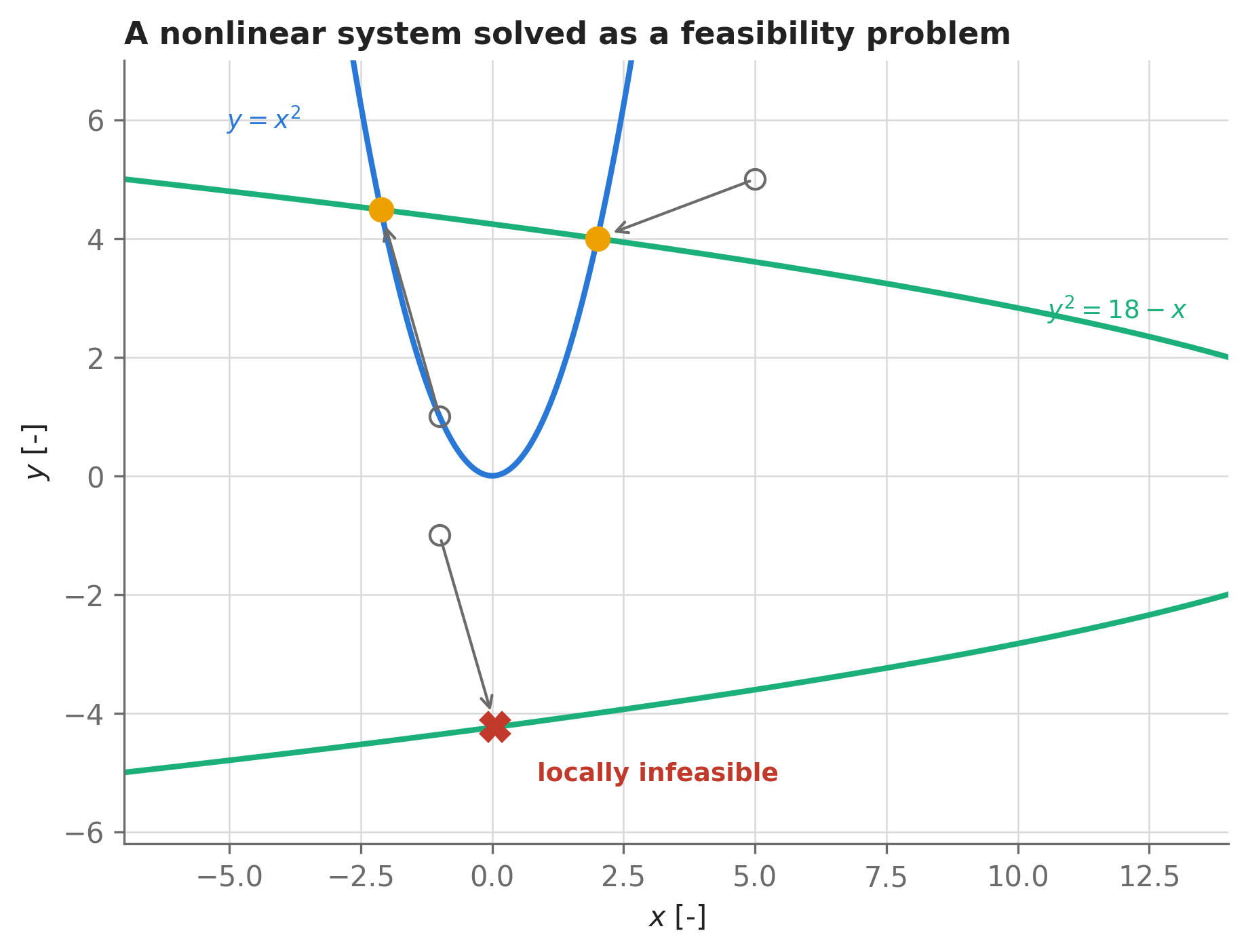
When is a pure feasibility problem well-posed? Essentially when the constraint Jacobian is square and full-rank — the same condition under which the nonlinear system has locally unique solutions. If you have fewer independent equality constraints than variables, the optimization framing degrades gracefully: add an objective and you’re doing least-squares-style closure on an underdetermined system, the nonlinear generalization of a pseudoinverse. This pattern — writing governing equations as constraints and letting the optimizer converge the analysis simultaneously with the design — is the Simultaneous Analysis and Design (SAND) architecture that powers the trajectory and aerostructural chapters later in this book.
5.7 When the solver fails
Solves fail. On well-scaled, NaN-safe problems (the craft of the previous chapter) they fail rarely — but you will still meet each of these, and each calls for a different response:
| Symptom | Likely cause | First move |
|---|---|---|
Infeasible_Problem_Detected |
Contradictory constraints, or a bad basin (as above) | Inspect the last iterate; sol.show_infeasibilities() |
Maximum_Iterations_Exceeded |
Poor problem scaling; genuinely hard nonconvexity | Re-scale variables/objective; better initial guess |
Restoration_Failed / Invalid_Number_Detected |
NaNs from sqrt/log/division of negative intermediates |
Domain-guard your model |
| Objective diverges to \(-\infty\) | Missing physics: nothing pushes back | Add the constraint or cost that reality would |
The key debugging affordance: even when no solution exists, the last iterate is always available. Two ways to get it: opti.debug.value(expression) works after a raised failure, and opti.solve(behavior_on_failure="return_last") skips the exception entirely and hands you the last iterate wrapped as a normal solution object (check sol.stats()["success"] before trusting it!).
Here’s the workflow on a physically infeasible variant of our cruise problem — a noise requirement caps airspeed at 20 m/s, but the airplane cannot generate 8000 N of lift that slowly:
opti = asb.Opti()

V = opti.variable(init_guess=30, scale=10)  # airspeed [m/s]
CL = opti.variable(init_guess=1.0)  # lift coefficient [-]

q = 0.5 * 1.225 * V**2
opti.subject_to(q * 10.0 * CL == 8000)  # lift = weight
opti.subject_to(CL <= 1.6)  # stall limit
opti.subject_to(V <= 20)  # noise-driven speed cap: physically too ambitious
opti.minimize(q * 10.0 * (0.030 + CL**2 / (np.pi * 8.0 * 0.90)) * V)

sol_bad = opti.solve(verbose=False, behavior_on_failure="return_last")

print(f"status:       {sol_bad.stats()['return_status']}")
print(f"last iterate: V = {sol_bad(V):.2f} m/s,  CL = {sol_bad(CL):.3f}")
status: Infeasible_Problem_Detected
last iterate: V = 20.00 m/s, CL = 3.265The last iterate already tells the story: the solver drove \(V\) to its 20 m/s cap and then cranked \(C_L\) to 3.27 trying to make lift — far beyond the stall limit. sol.show_infeasibilities() makes the diagnosis explicit, printing every violated constraint with the source line that created it:
sol_bad.show_infeasibilities(tol=1e-3)--------------------------------------------------
3.265306057143619 < 1.6 (violation: 1.665306057143619)
Scalar constraint defined in `4272270844.py`, line 8:
```
opti.subject_to(CL <= 1.6) # stall limit
```That source-traceback machinery (opti.find_constraint_declaration() and find_variable_declaration() underneath) is worth remembering on thousand-constraint problems, where “constraint #847 is violated” is useless but “the stall constraint from line 12 of wing.py is violated by 1.67” is a diagnosis. From here the resolution is an engineering decision, not a numerical one: relax the speed cap, add wing area, or shed weight — and after re-solving, the duals from Section 5.4 will tell you exactly what each option is worth. For a fuller decision tree (scaling pathologies, NaN forensics, and more exotic IPOPT exit codes), see the FAQ / troubleshooting appendix.
5.8 Where to go next
- These tools compound on real problems: the SimPleAC aircraft-sizing chapter uses dual-based sensitivities on a full conceptual design, reproducing (and out-running) a geometric-programming benchmark.
- If your solves are slow or flaky, the cure is almost always in the model, not the solver: revisit the chapter on building robust optimization models.
- The
parameter+ sweep + warm-start pattern reappears at scale in the trajectory-optimization chapters, where continuation along a parameter is often the practical path to convergence.