Half of using an optimizer well is writing models that the optimizer can chew. This chapter teaches you to recognize and fix the three failure modes that account for nearly every “my solve failed” moment in practice: kinks (functions that aren’t smoothly differentiable), NaNs (functions evaluated outside their domain), and bad scaling (variables whose magnitudes differ by many orders of magnitude). Each one gets a minimal failing example, an explanation of why the solver chokes, and a toolbox of fixes — exact reformulations, the smooth-approximation functions built into aerosandbox.numpy, and the scale= and log_transform= arguments of opti.variable(). By the end, you’ll be able to read a solver failure the way a mechanic reads an engine noise. If you’ve landed here from a failed solve and want the quick diagnosis first, jump to the checklist in Section 3.5.
3.1 How the optimizer sees your model
When you call opti.solve(), AeroSandbox hands your problem to IPOPT, a second-order gradient-based optimizer, with exact first and second derivatives computed by the CasADi automatic-differentiation engine. At every iteration, IPOPT builds a local quadratic model of your objective and constraints from those derivatives, solves it to get a search direction, and steps. This machinery is extraordinarily effective — it’s what lets AeroSandbox solve problems with thousands of design variables in seconds — but it rests on three assumptions about your model:
Smoothness. The objective and constraints should be continuously differentiable (ideally twice, i.e., \(C^2\)), so that a local quadratic model exists everywhere.
Finiteness. Every function and its derivatives must evaluate to a finite number at every point the optimizer might visit — which is a much bigger set than the feasible region. Interior-point methods probe infeasible points constantly during the solve, so your model must survive evaluation off the constraint manifold, not just on it.
Reasonable scale. After scaling, variables and functions should live within a few orders of magnitude of 1, so that floating-point arithmetic on the internal linear algebra stays well-conditioned.
Violate any of these and the solver will slow down, stall, or crash — usually with an error message that makes sense only once you know which assumption you broke. Let’s break each one on purpose.
3.2 Kinks: continuity and differentiability
The takeaway: if your objective or constraints have a kink — a point where the first derivative jumps — the optimizer can fail even when the problem looks trivial. Here is the smallest possible demonstration: minimize \(|x|\). The answer is obviously \(x = 0\), and the setup could hardly be simpler:
import aerosandbox as asbimport aerosandbox.numpy as npopti = asb.Opti()x = opti.variable(init_guess=1)opti.minimize(np.fabs(x))try: sol = opti.solve(verbose=False)exceptRuntimeError:print("Solver failed!")print(f" Return status: {opti.debug.stats()['return_status']}")print(f" Last iterate: x = {opti.debug.value(x):.6e}")
Solver failed!
  Return status: Error_In_Step_Computation
  Last iterate:  x = 1.084681e-06
Two things are worth noticing in the wreckage. First, the failure diagnostics: after any failed solve, opti.debug.value(x) retrieves the last value of any variable or expression before the solver gave up, and opti.debug.stats() reports IPOPT’s exit status — both are your first stop when debugging. Second, where it died: the last iterate is within about \(10^{-6}\) of the true optimum. The solver marched happily toward \(x = 0\), and then its line search disintegrated on final approach. That signature — near-convergence followed by Error_In_Step_Computation or Restoration_Failed — is the classic fingerprint of a kink at the optimum.
Why does this happen? IPOPT’s local quadratic model needs a finite second derivative. Away from \(x=0\), \(|x|\) is just a straight line and the model is fine. But at the kink, the slope jumps from \(-1\) to \(+1\) over zero distance: the curvature there is effectively infinite, no finite quadratic can represent it, and the step computation breaks down exactly where the optimizer most needs it to work. Hence the rule of thumb:
Keep your objective and constraints \(C^1\)-continuous (continuous, with continuous first derivatives). You can sometimes get away with a kink if the optimizer never visits it — but a kink at or near the optimum is almost always fatal.
3.2.1 Fix 1: reformulate the kink away exactly
The best fix, when available, changes the problem algebraically without changing its solution. Note that \(|x| = \max(x, -x)\): a max of two smooth functions. Whenever you’re minimizing (or upper-bounding) such a max, you can introduce an auxiliary variable that sits above every branch, and minimize the auxiliary variable instead — the optimizer pulls it down until it touches whichever branch is active:
opti = asb.Opti()x = opti.variable(init_guess=1)t = opti.variable(init_guess=1) # auxiliary variable: t will equal max(x, -x)opti.subject_to([ t >= x, t >=-x,])opti.minimize(t)sol = opti.solve(verbose=False)print(f"x = {sol(x):.2e}, solved in {sol.stats()['iter_count']} iterations")
x = 6.09e-10, solved in 4 iterations
Every function the solver now sees is linear — no kinks anywhere — and the problem solves in a handful of iterations. This epigraph reformulation is exact: no approximation error, no tuning parameters. Use it whenever a max (or a min that you’re maximizing or lower-bounding) appears in a convex position in your problem.
It can’t do everything, though. Consider a genuinely piecewise function like
\[
f(x) =
\begin{cases}
-x & x < 0\\
(x-1)^2 - 1 & x \geq 0,
\end{cases}
\]
which is neither the max nor the min of its two branches — no auxiliary-variable trick can represent it exactly with smooth constraints. For cases like this, we approximate.
3.2.2 Fix 2: smooth the kink
The second strategy replaces the kinked function with a smooth one that’s close to it. Be clear-eyed about what this means: you are now solving a slightly different problem, and the optimum will shift by an amount controlled by how aggressively you smooth. The trade is usually excellent — engineering models carry percent-level uncertainty anyway, and a smooth model that solves reliably beats an exact model that crashes.
aerosandbox.numpy ships two general-purpose smoothers, one for each of the two kinds of kink you’ll meet:
np.softmax(*args, softness=s) — a smooth, convexity-preserving replacement for max() (and np.softmin for min()). It’s the log-sum-exp function: with words first — it returns roughly the largest of its arguments, erring slightly high, with the error largest when arguments are nearly tied. Symbolically: \[
\mathrm{softmax}(x_1, \ldots, x_n) = s \, \ln\!\left(\sum_i e^{x_i / s}\right),
\] which satisfies \(\max_i x_i \;\leq\; \mathrm{softmax} \;\leq\; \max_i x_i + s \ln n\). The softness\(s\) has the same units as the inputs: choose it as the size of discrepancy between the inputs that you’d consider physically negligible. (An equivalent hardness=1/s argument also exists, as does np.softmax_scalefree, which picks \(s\) automatically relative to the input magnitudes.)
np.blend(switch, value_high, value_low) — a smooth replacement for np.where(condition, value_if_true, value_if_false). Instead of a hard boolean, it takes a continuous switch value and fades between the two branches with a sigmoid: strongly positive switch returns value_high, strongly negative returns value_low, and the transition has width of order \(\pm 1\) in switch units (so np.blend(x / width, hi, lo) gives you control of the crossover sharpness). Blend handles arbitrary piecewise functions — but, unlike softmax, it does not preserve convexity.
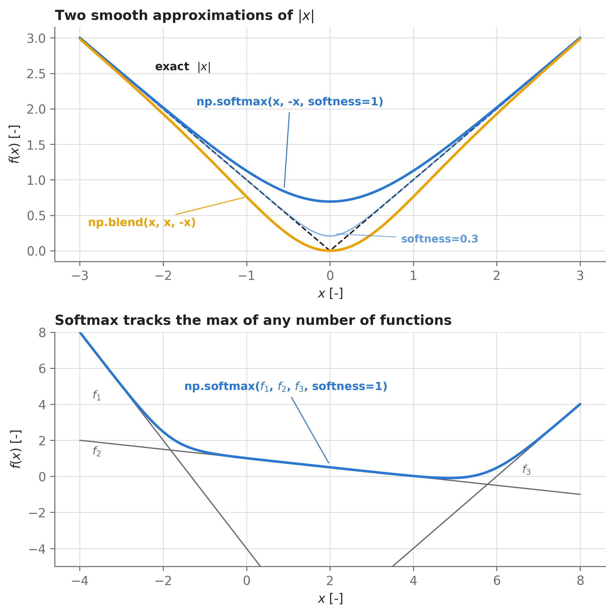
Both applied to our absolute-value example — \(|x| = \max(x, -x) = \mathrm{where}(x > 0,\ x,\ -x)\) — look like this:
Figure 3.1: Smooth stand-ins for kinked functions. Top: two library one-liners approximating |x|; softmax errs high near the kink (by at most softness × ln 2), while blend errs low. Bottom: softmax generalizes to any number of functions, tracking the max of three cost lines with one smooth curve.
Both curves in the top panel of Figure 3.1 would sail through the optimizer. So why prefer one over the other?
3.2.3 Convexity is worth protecting
The difference between the two smoothers is invisible in Figure 3.1 but decisive in practice: softmax preserves convexity, blend doesn’t. Convexity is what guarantees that a function has no spurious local minima — and IPOPT, like every practical large-scale optimizer, is a local optimizer. It converges to a minimum; convex structure is what promises that minimum is the minimum.
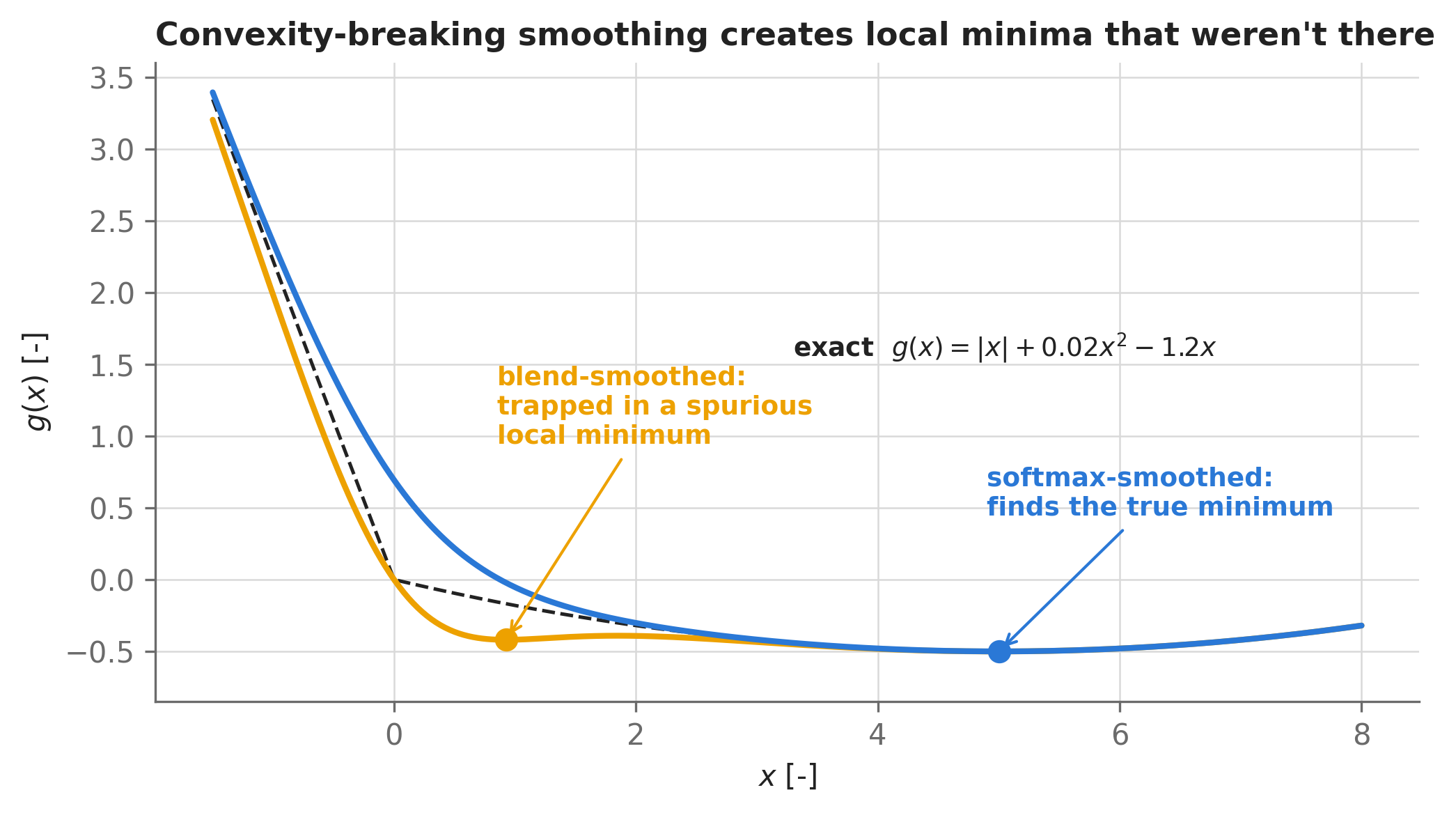
To see the danger concretely, embed our smoothed \(|x|\) inside a slightly larger problem: minimize \(g(x) = |x| + 0.02x^2 - 1.2x\). The exact \(g\) is convex (a sum of convex functions), with a unique minimum near \(x = 5\). Now smooth the \(|x|\) term both ways and let the optimizer loose from \(x_0 = 0\):
Figure 3.2: The same convex problem, smoothed two ways. Blend’s convexity-breaking approximation carves a spurious dip near the old kink, and the optimizer falls in; softmax’s convexity-preserving approximation keeps the design space unimodal and lands on the true optimum. Dots mark where each solve actually converged.
The blend-based smoothing turned a unimodal problem into a multimodal one (Figure 3.2), and the optimizer converged — cleanly, confidently, with a happy exit status — to an answer that is wrong by a factor of five. Nothing in the solver output warns you. This is why the choice of smoother matters:
When smoothing a max-like or min-like kink, use np.softmax/np.softmin — they preserve convexity. Reach for np.blend only for genuinely piecewise switches that softmax can’t represent, and treat the result as potentially multimodal (e.g., try multiple initial guesses).
And blend does earn its keep on those genuine switches. The piecewise function from earlier — where the epigraph trick was powerless — smooths and solves in one line each:
opti = asb.Opti()x = opti.variable(init_guess=-2) # start on the far branchf_smooth = np.blend(4* x, # switch: crossover of width ~1/4 around x = 0 (x -1)**2-1, # branch used where the switch is strongly positive-x, # branch used where the switch is strongly negative)opti.minimize(f_smooth)sol = opti.solve(verbose=False)print(f"x = {sol(x):.4f} (exact minimum is at x = 1)")
x = 1.0002 (exact minimum is at x = 1)
Two practical notes on smoothing. First, the smoothing parameter is a knob between fidelity and solvability: as softness shrinks toward zero, the approximation error vanishes but the curvature at the old kink grows — take it too far and you’ve rebuilt the original pathology. Second, a useful pattern when you need high fidelity is continuation: solve once with generous softness, then re-solve with it tightened, warm-starting from the previous solution.
Finally, keep a mental watch-list of the innocuous-looking functions that put kinks (or worse) into models:
If your model uses…
The hazard
Robust alternative
np.fabs(x)
kink at \(x=0\)
epigraph reformulation, or np.softmax(x, -x)
np.fmax(a, b), np.fmin(a, b)
kink wherever \(a = b\)
np.softmax(a, b), np.softmin(a, b)
np.where(cond, a, b)
jump or kink at the switch
np.blend(switch, a, b)
clipping at zero, e.g. \(\max(x,0)\)
kink at the clip
np.softplus(x, beta=...)
np.floor, np.round, table lookups with switching
zero gradient almost everywhere — the optimizer is blind
The takeaway: a NaN anywhere in your model — in a function value or any derivative — blinds the optimizer completely, and constraints alone will not keep you out of NaN territory. A kink degrades the solver’s information; a NaN erases it. With no objective value and no gradient, IPOPT doesn’t know how good the current point is or which direction leads back to safety.
The usual culprits are functions with restricted domains:
\(\sqrt{x}\) with \(x < 0\) — and more generally \(x^p\) for non-integer \(p\),
\(\ln(x)\) with \(x \leq 0\),
division \(a/b\) as \(b \to 0\) (an Inf, equally fatal),
np.arcsin / np.arccos outside \([-1, 1]\),
and, more subtly, functions whose derivative is infinite somewhere — \(\sqrt{x}\) again, whose slope blows up as \(x \to 0^+\).
Start with the blunt case: minimize \(\sqrt{x}\) from an initial guess of \(x = -1\). The very first gradient evaluation happens at the initial guess, returns NaN, and IPOPT refuses to take a single step:
opti = asb.Opti()x = opti.variable(init_guess=-1)opti.minimize(np.sqrt(x))try: sol = opti.solve(verbose=False)exceptRuntimeError:print(f"Return status: {opti.debug.stats()['return_status']}")
Return status: Invalid_Number_Detected
Invalid_Number_Detected at iteration zero almost always means exactly this: your initial guess produces a NaN somewhere in the model. Check the guesses first.
Now the subtle case. Fix the initial guess and add the “obvious” constraint:
opti = asb.Opti()x = opti.variable( init_guess=1, lower_bound=0, # shorthand for opti.subject_to(x >= 0))opti.minimize(np.sqrt(x))try: sol = opti.solve(verbose=False)exceptRuntimeError:print(f"Return status: {opti.debug.stats()['return_status']}")print(f"Last iterate: x = {opti.debug.value(x):.2e}")
Return status: Error_In_Step_Computation
Last iterate:  x = 2.25e-15
The problem now looks mathematically well-posed — minimize a function over exactly its domain — yet it still fails, for two compounding reasons:
The gradient is infinite at the solution.\(d(\sqrt{x})/dx = 1/(2\sqrt{x}) \to \infty\) as \(x \to 0^+\), and the minimum sits precisely at \(x = 0\). The quadratic model degenerates on final approach, just as it did at the kink.
Constraints are not fences. IPOPT deliberately relaxes bounds by a small amount (its bound_relax_factor, default \(10^{-8}\)) because doing so improves performance on well-behaved problems. So even a “feasible” iterate may sit at \(x \approx -10^{-8}\) — and your model must survive being evaluated there. A constraint keeps the converged answer essentially feasible; it does not keep every intermediate evaluation inside your function’s domain.
Point 2 is worth internalizing as a general design principle for optimization-ready models: your model should return finite values and gradients in a neighborhood of the feasible region, not just inside it. Here are four ways to achieve that, roughly in order of preference.
Fix 1: eliminate the dangerous function algebraically. Often the cleanest move. Monotonic transformations don’t change which point is optimal, so opti.minimize(np.sqrt(f)) can simply become opti.minimize(f) (when \(f \geq 0\)). The same idea rewrites constraints: instead of \(\sqrt{x^2 + y^2} \leq R\), write \(x^2 + y^2 \leq R^2\); instead of \(\ln(x) \geq c\), write \(x \geq e^c\). No approximation, no NaN surface anywhere. For our toy problem, minimizing \(x\) itself gives the identical answer with no square root in sight.
Fix 2: leave a buffer at domain boundaries. When the domain edge is genuinely off-limits (it usually is, physically — a wing with zero chord isn’t a design, it’s a division by zero), set the bound a small distance inside the domain, so the solver’s \(\sim 10^{-8}\) boundary slop never reaches the singularity:
opti = asb.Opti()x = opti.variable(init_guess=1, lower_bound=1e-6) # buffer, not exactly 0opti.minimize(np.sqrt(x))sol = opti.solve(verbose=False)print(f"x = {sol(x):.2e}, solved in {sol.stats()['iter_count']} iterations")
x = 9.90e-07, solved in 13 iterations
Pick the buffer small compared to physically meaningful values of the variable but large compared to \(10^{-8}\) — for a chord length in meters, lower_bound=1e-3 is plenty safe.
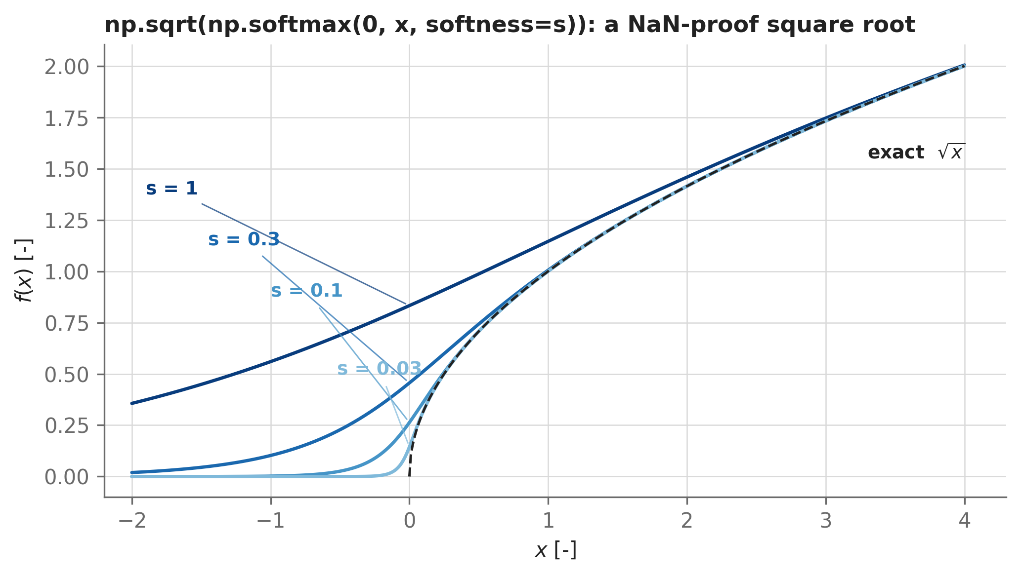
Fix 3: guard the argument with a smooth clamp. The smoothing tools from Section 3.2.2 double as domain guards: np.softmax(0, x, softness=s) is a convexity-preserving “soft clamp” that stays strictly positive for all \(x\), with finite slope everywhere, and tracks \(x\) ever more closely as the softness shrinks:
Figure 3.3: A softmax guard makes sqrt safe: sqrt(softmax(0, x, softness=s)) is defined and has finite gradients for all x — even negative x — and converges to the exact square root as the softness shrinks.
The guarded model (Figure 3.3) is evaluable on the entire real line, so no amount of solver wandering can produce a NaN.
Fix 4: make positivity structural with log_transform=True. For quantities that are physically positive — masses, areas, densities, velocities-squared — you can tell the optimizer to work with \(\ln(x)\) internally:
Closed design: mass_total = 209.4 kg (6 iterations)
Since the solver’s internal variable is \(z = \ln(m)\) and your model sees \(m = e^z\), no iterate can ever be negative — the non-integer power mass_total**1.05 above is unconditionally NaN-safe. This little weight-closure model finds that carrying a 100 kg payload requires a 209 kg vehicle. Log-transforming has a second benefit we’ll meet in the next section: it automatically fixes scaling for variables that span decades, and it makes power-law models (which fill aircraft design) linear in the transformed space. Its costs: the initial guess must be positive, and expressions that were convex in \(x\) aren’t always convex in \(\ln x\), so treat it as a tool for positive, multiplicative-flavored quantities rather than a default.
3.4 Scaling: keep everything near 1
The takeaway: the single cheapest speedup in all of asb.Opti is telling the optimizer roughly how big your variables are. Engineering problems mix quantities like a skin gauge of \(10^{-4}\) m and a modulus of \(7 \times 10^{10}\) Pa — fourteen orders of magnitude in one Hessian. Newton’s method is scale-invariant on paper, but in float64 arithmetic that Hessian is numerically garbage, and several of IPOPT’s internal heuristics (regularization, bound handling) are not scale-invariant at all. The result is a solver that limps: hundreds of iterations, tiny steps, or outright failure, on problems that are mathematically easy.
AeroSandbox’s convention: opti.variable(..., scale=s) divides the variable by \(s\) internally, so the optimizer works with numbers of order 1. If you don’t pass scale, AeroSandbox auto-scales using the mean magnitude of your init_guess — which means good initial guesses buy you good scaling for free, and which also sets up the trap we’re about to walk into: an initial guess of zero contains no magnitude information, so the auto-scaling heuristic falls back toscale=1.
Let’s see the whole story on a classic problem, adapted from the CasADi blog’s scaling case study: a 1-D rocket that must reach 100 km altitude at \(t = 100\) s while burning minimum propellant, written — as good SI-respecting engineers would — in meters, kilograms, and newtons.
import time### Problem constantsN =100# number of discretization pointstime_final =100# [s] fixed flight durationt = np.linspace(0, time_final, N) # [s] time gridmass_launch =500e3# [kg] launch massaltitude_final =100e3# [m] target altitudeg =9.81# [m/s^2] gravitational accelerationalpha =1/ (300* g) # [kg/N/s] propellant burned per N of thrust (Isp = 300 s)def solve_rocket(init_guesses: dict, scales: dict|None=None) -> asb.OptiSol:"""Minimum-propellant 1-D rocket ascent, transcribed via forward Euler.""" opti = asb.Opti() scales = scales or {} altitude = opti.variable(init_guess=init_guesses["altitude"], n_vars=N, scale=scales.get("altitude")) # [m] velocity = opti.variable(init_guess=init_guesses["velocity"], n_vars=N, scale=scales.get("velocity")) # [m/s] mass = opti.variable(init_guess=init_guesses["mass"], n_vars=N, scale=scales.get("mass")) # [kg] thrust = opti.variable(init_guess=init_guesses["thrust"], n_vars=N, scale=scales.get("thrust")) # [N] opti.subject_to([ # Dynamics, discretized by forward Euler: np.diff(altitude) == velocity[:-1] * np.diff(t), np.diff(velocity) == (thrust[:-1] / mass[:-1] - g) * np.diff(t), np.diff(mass) ==-alpha * thrust[:-1] * np.diff(t), ]) opti.subject_to([ # Boundary conditions: altitude[0] ==0, velocity[0] ==0, mass[0] == mass_launch, altitude[-1] == altitude_final, ]) opti.subject_to([mass >=0, thrust >=0]) # Path constraints opti.minimize(-mass[-1]) # max final mass == min propellant burned sol = opti.solve(verbose=False, max_iter=2000) sol.arrays = { # stash the trajectory for plotting k: sol(v) for k, v indict(altitude=altitude, velocity=velocity, mass=mass, thrust=thrust).items() }return sol
First, solve it the way an experienced user would — with rough physics-based initial guesses (a linear climb, the average climb rate, launch mass, hover-ish thrust):
guess_from_physics =dict( altitude=np.linspace(0, altitude_final, N), # linear climb to target velocity=altitude_final / time_final, # average climb rate mass=mass_launch, thrust=g * mass_launch, # ballpark: hover thrust)sol_good = solve_rocket(guess_from_physics)iters_good = sol_good.stats()["iter_count"]print(f"Solved in {iters_good} iterations.")
Solved in 12 iterations.
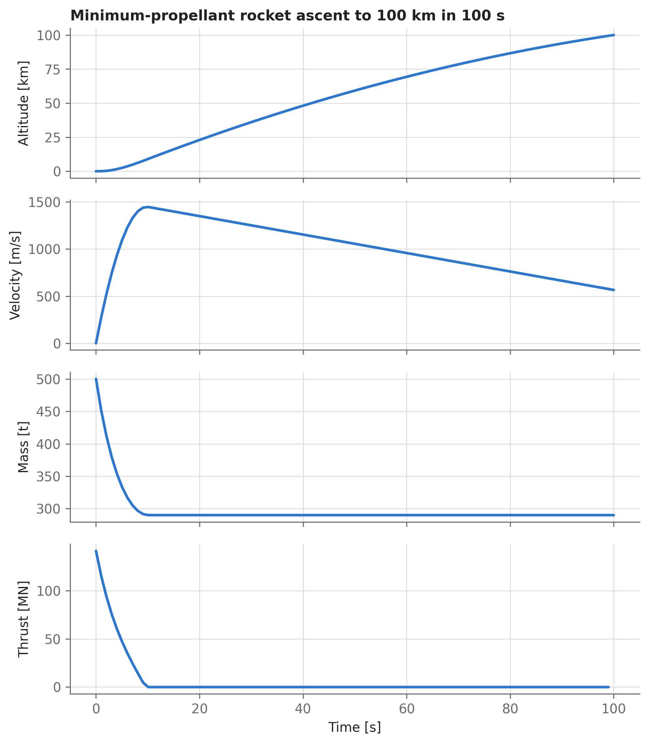
Figure 3.4: The minimum-propellant ascent: with no thrust ceiling in the model, the optimizer burns hard and early (nearly impulsively), then coasts to arrive at 100 km exactly at t = 100 s.
12 iterations — snappy. Under the hood, those representative initial guesses did double duty: they started the solver in the right neighborhood, and they fed the auto-scaling heuristic sensible magnitudes (\(\sim 10^5\) for altitude in meters, \(\sim 10^5\) for mass in kilograms, and so on).
Now the trap. Suppose we’d initialized the trajectory the lazy way — “the rocket starts at rest on the pad, so let’s just guess zero for everything that starts at zero”:
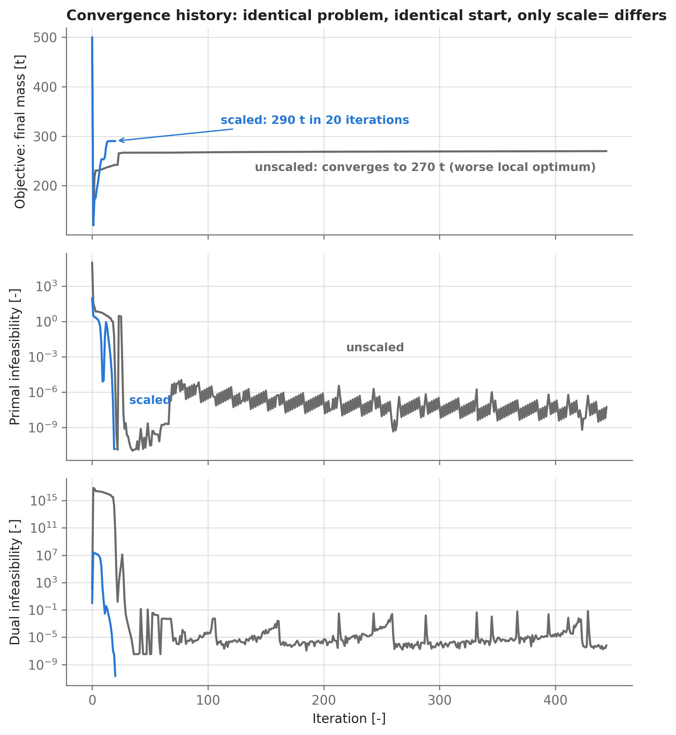
Same physics, same constraints — but the solve grinds through 444 iterations instead of 12. The zero guesses gave the auto-scaler nothing to work with, so a 100,000-meter altitude and a meganewton-class thrust are both being treated as order-1 quantities. (A poor starting point costs something too, but as we’re about to see, it’s a minor charge next to the scaling damage.) And the slowness turns out not even to be the worst of it — hold that thought for one code block.
The fix costs four lines. Keep the identical lazy initial guesses, and just tell the optimizer the characteristic magnitude of each variable — order-of-magnitude honesty is all that’s required:
scales =dict( altitude=1e5, # [m] ~100 km of climb velocity=1e3, # [m/s] ~km/s-class speeds mass=5e5, # [kg] ~launch mass thrust=5e6, # [N] ~weight of the vehicle)tic = time.perf_counter()sol_scaled = solve_rocket(guess_zeros, scales)t_scaled = time.perf_counter() - ticiters_scaled = sol_scaled.stats()["iter_count"]print(f"Solved in {iters_scaled} iterations ({t_scaled:.2f} s).")
Solved in 20 iterations (0.18 s).
Starting from the same point in the design space, the well-scaled problem converges in 20 iterations versus 444 — about 22× fewer — and the wall-clock speedup on this machine is roughly 23×. But compare the two answers, and something more disturbing than slowness appears: the trajectories disagree. This problem is nonconvex (thrust and mass multiply each other in the dynamics), so it admits multiple local optima — and the ill-conditioned solve didn’t just crawl, it crawled into a worse basin, converging with a clean exit status to a trajectory that burns 10% more propellant. The well-scaled solve, from the identical all-zeros start, recovers the same optimum as the physics-guessed run (relative difference: 3e-13). Figure 3.5 shows both effects from inside the solver:
Figure 3.5: IPOPT convergence history for the two zero-guess rocket solves — identical problem, identical start, only scale= differs. The scaled solve (blue) converges almost immediately; the unscaled solve (gray) grinds through hundreds of ill-conditioned iterations and settles into a worse local optimum (top panel).
Let that sink in: bad scaling costs you speed at best, and answer quality at worst — and the second failure mode is silent. Distilled into working rules:
Aim for scaled magnitudes between roughly 0.01 and 100.scale is a unit choice, not a precision claim — being right to within an order of magnitude captures nearly all the benefit.
Give representative (nonzero!) initial guesses and auto-scaling handles the rest. The heuristic is scale = mean(abs(init_guess)). It fails exactly when the guess is zero or wildly unrepresentative of the converged magnitude — those are the cases where you must pass scale= yourself.
Variables are your job; functions are mostly IPOPT’s. IPOPT auto-scales the objective and constraints using their gradients at the initial guess (its default nlp_scaling_method="gradient-based"), but it never rescales your variables. That said, keeping constraint residuals near order 1 (e.g., writing a force balance in meganewtons rather than newtons, or normalizing: opti.subject_to(L / W == 1) instead of L == W) removes any dependence on that heuristic.
For positive quantities spanning decades, log_transform=True is auto-scaling. In log-space, a wing loading of \(10^2\) and a modulus of \(10^{11}\) become 4.6 and 25.3 — neighbors.
3.5 When a solve fails: a field guide
Everything in this chapter compresses into a diagnostic table. When opti.solve() throws, read the return_status (it’s in the exception message, and in opti.debug.stats()["return_status"]), pull the last iterate with opti.debug.value(...), and look up the signature:
Symptom
Most likely cause
First fix to try
Invalid_Number_Detected, dies at iteration 0
Initial guess produces NaN/Inf in the model
Evaluate your model by hand at the initial guesses; fix guesses or domains (Section 3.3)
Invalid_Number_Detected, dies mid-solve
An iterate wandered outside a function’s domain
Buffer the domain bounds; add smooth guards; log_transform=True (Section 3.3)
Error_In_Step_Computation / Restoration_Failed near an apparent optimum
Solves quickly and confidently… to a suspicious answer
Multimodality (perhaps introduced by a convexity-breaking smoother)
Re-solve from several initial guesses; prefer np.softmax over np.blend (Section 3.2.3)
Two habits make these failures rare in the first place. Write models that are evaluable everywhere, not just at feasible points — buffered bounds, softmax guards, log-transformed positives. And give every variable an honest initial guess, which simultaneously sets the starting point and the scaling. Models built this way don’t just fail less; they solve faster, because the optimizer spends its iterations on your physics instead of on numerical pathology.
3.6 Where to go next
The solver itself is the subject of the next chapter: reading IPOPT’s iteration log (Section 5.2), adjusting solver options (Section 5.3), extracting parametric sensitivities (Section 5.4), and the full opti.debug failure workflow (Section 5.7).
These robustness patterns pay off the moment models get physical: the wing design case study (Section 10.1) puts them to work on real aircraft trade studies.
For a symptom-indexed troubleshooting list (including IPOPT return codes not covered here), see the FAQ appendix.