Appendix A — A Map of the API

This appendix is the orientation guide to AeroSandbox’s public API. You will learn how the namespace is organized (so you know where to look for things), where the complete auto-generated reference documentation lives, how to decode the docstring and type-hint conventions used throughout the library, and what the versioning policy promises when you upgrade. It is deliberately short: the full per-function reference is generated straight from the source code and lives online, so this chapter teaches you how to navigate that documentation rather than duplicating it.

A.1 One import, three namespaces

Nearly everything you use in day-to-day AeroSandbox work is reachable through three imports:

import aerosandbox as asb             # all major classes: Opti, Airplane, AeroBuildup, ...
import aerosandbox.numpy as np        # drop-in NumPy that also accepts optimization variables
import aerosandbox.tools.units as u   # unit-conversion factors: u.knot, u.lbm, u.foot, ...

The asb namespace is intentionally flat: every major class is exported at the top level, so code reads as asb.Wing, not aerosandbox.geometry.wing.Wing. The table below lists every top-level export, grouped by discipline — it is generated live by introspecting the installed library at render time, so it cannot go stale.

Table A.1: All 46 top-level exports of the aerosandbox namespace, generated by introspecting version 4.2.9 at render time.

Discipline	Top-level exports (asb.<name>)
Optimization	Opti, OptiSol
Geometry	Airfoil, Airplane, ControlSurface, Fuselage, FuselageXSec, KulfanAirfoil, Propulsor, Wing, WingXSec, reflect_over_XZ_plane
Aerodynamics analyses	AVL, AeroBuildup, AirfoilInviscid, LiftingLine, MSES, NonlinearLiftingLine, VortexLatticeMethod, XFoil
Atmosphere	Atmosphere
Operating point	OperatingPoint
Flight dynamics	DynamicsPointMass1DHorizontal, DynamicsPointMass1DVertical, DynamicsPointMass2DCartesian, DynamicsPointMass2DSpeedGamma, DynamicsPointMass3DCartesian, DynamicsPointMass3DSpeedGammaTrack, DynamicsRigidBody2DBody, DynamicsRigidBody3DBodyEuler
Mass properties	MassProperties, mass_properties_from_radius_of_gyration, mass_properties_of_cube, mass_properties_of_ellipsoid, mass_properties_of_rectangular_prism, mass_properties_of_sphere
Surrogate modeling	FittedModel, InterpolatedModel, UnstructuredInterpolatedModel, black_box
Framework base classes	AeroSandboxObject, ExplicitAnalysis, ImplicitAnalysis, load
Utilities	docs, run_tests

The other two imports are conventions you will see in every chapter of this book. aerosandbox.numpy re-exports all of NumPy, with trace-breaking functions rewritten so they work on both plain arrays and optimization variables (Optimization Basics explains why). aerosandbox.tools.units is a module of plain floats — multiplicative conversion factors to base SI units — so airspeed = 100 * u.knot gives meters per second.

A.2 The subpackage map

Anything not in Table A.1 is imported from its subpackage (e.g., from aerosandbox.library import propulsion_turbofan). There are fourteen subpackages; the two under “core” are the ones the library’s own documentation says get you 90% of the way there.

Table A.2: The AeroSandbox subpackage map.

Subpackage	What lives there	Covered in
optimization	Core. The Opti stack: an object-oriented way to formulate and solve engineering optimization problems.	Optimization Basics
numpy	Core. The drop-in NumPy replacement that preserves the automatic-differentiation trace.	Optimization Basics
geometry	Object-oriented aircraft geometry — Airplane, Wing, Fuselage, Airfoil, and friends — plus 3D drawing and CAD export.	Geometry
aerodynamics	2D and 3D aerodynamics analyses: AeroBuildup, VortexLatticeMethod, lifting-line methods, and wrappers for XFoil, AVL, and MSES.	Airfoil & Aircraft Aerodynamics, External Tools
atmosphere	Standard-atmosphere models: the ISA, and a differentiable fit to it.	Atmosphere, Propulsion & Weights
performance	OperatingPoint: the flight condition (atmosphere, speed, alpha, beta, rotation rates) an airplane is analyzed at.	Atmosphere, Propulsion & Weights
dynamics	The flight-dynamics engine: point-mass and rigid-body models for simulating and optimizing trajectories.	The Dynamics Stack
structures	Beam models (tube_spar_bending) and buckling criteria (buckling).	Structures
weights	MassProperties (mass, CG, inertia tensor, with an algebra for combining them) and mass properties of simple shapes.	Atmosphere, Propulsion & Weights
propulsion	A placeholder, currently work-in-progress; today’s propulsion models live in library.	—
library	Ready-made surrogate models by the hundred: propulsion (propulsion_electric, propulsion_turbofan, …), power systems (power_solar, …), structural mass, aerodynamics, costs, winds, field lengths. Some physics-based, some empirical fits; each documents its units and sources in its docstring.	Atmosphere, Propulsion & Weights, Solar UAV Sizing
modeling	Build-your-own surrogates: FittedModel, InterpolatedModel, black_box.	Surrogate Modeling
tools	Standalone utilities: units, pretty_plots, string formatting, benchmarking.	used throughout
visualization	Plotting machinery behind the .draw() methods.	—

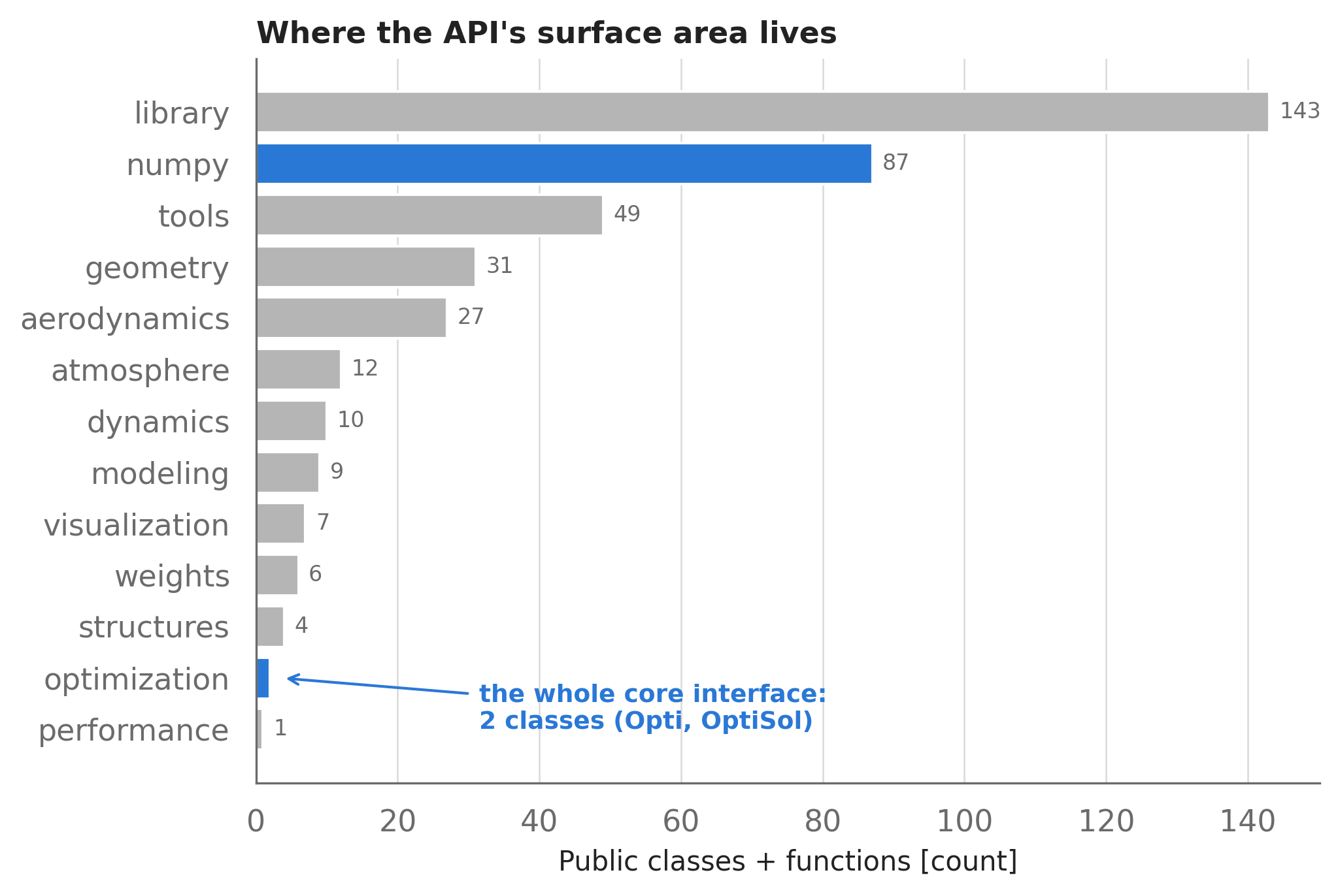
To give you a quantitative feel for where the library’s surface area actually is, Figure A.1 counts the public classes and functions defined in each subpackage — again computed live against the installed version.

Figure A.1: Public API surface area by subpackage, counted by introspection at render time. The largest subpackage by far is the library of ready-made surrogate models; the core optimization interface you must actually learn is just two classes.

The shape of this chart is the design philosophy of the library in one picture: a tiny core you must learn (optimization is literally two classes — highlighted in blue, along with the numpy shim that makes your models differentiable), surrounded by a large, optional collection of physics models and utilities you dip into as needed.

A.3 Where the full reference lives

Three places, in decreasing order of formality:

1. The reference website: aerosandbox.readthedocs.io. Complete API documentation for every public module, class, and function, auto-generated from the source docstrings (via sphinx-autoapi) — so it is always in sync with the code. This is the place to browse signatures and options for a class you already know you need.
2. help() in your Python session. Every public object is documented in-source, so help(asb.Airplane) or help(asb.Opti.variable) prints the same documentation without leaving your terminal. There is also asb.docs(), which opens the project website in your browser.
3. The source itself: github.com/peterdsharpe/AeroSandbox. AeroSandbox is documented extensively in-source, and each subpackage ships its unit tests alongside the code (the test_* folders) — hundreds of small, runnable usage examples. When you wonder “how am I supposed to call this?”, the tests are often the fastest answer.

A.4 Reading docstrings and type hints

Docstrings state the units of every physical input and output. The library-wide default is base SI units (m, kg, s, N, Pa, W, J), with one long-standing aerospace exception: angle of attack alpha and sideslip beta are in degrees (all other angles are radians). Here is a representative docstring — note that every physical argument says what unit it expects:

import aerosandbox as asb
import inspect

print(inspect.getdoc(asb.Atmosphere.__init__))  # or just: help(asb.Atmosphere)

Initialize a new Atmosphere.

Args:

    altitude: Flight altitude, in meters. This is assumed to be a geopotential altitude above MSL.

    method: Method of atmosphere modeling to use. Either:
        * "differentiable" - a C1-continuous fit to the International Standard Atmosphere; useful for optimization.
            Mean absolute error of pressure relative to the ISA is 0.02% over 0-100 km altitude range.
        * "isa" - the International Standard Atmosphere, exactly reproduced

    temperature_deviation: A deviation from the temperature model, in Kelvin (or equivalently, Celsius). This is useful for modeling
        the impact of temperature on density altitude, for example.

Type hints tell you what a parameter accepts — including whether it can be symbolic. Look at the hint on that same altitude parameter:

print(inspect.signature(asb.Atmosphere.__init__).parameters["altitude"])

altitude: int | float | numpy.integer | numpy.floating | numpy.ndarray | casadi.casadi.MX | casadi.casadi.DM = 0.0

That union looks intimidating, but it decodes to exactly two facts. Everything up through numpy.ndarray says the parameter is vectorizable: pass a scalar for one flight condition or an array for many. The casadi.MX | casadi.DM tail says the parameter is hybrid: it also accepts an optimization variable, meaning you can put this model inside an asb.Opti problem and differentiate through it. All three modes, live:

import aerosandbox.numpy as np

print(asb.Atmosphere(altitude=11e3).pressure())  # scalar in, scalar out [Pa]

print(asb.Atmosphere(altitude=np.array([0, 10e3, 20e3])).pressure())  # vectorized [Pa]

opti = asb.Opti()
altitude = opti.variable(init_guess=10e3)
pressure = asb.Atmosphere(altitude=altitude).pressure()
print(type(pressure))  # symbolic: an expression the optimizer can differentiate

22645.178581886557
[101324.99999999  26436.26759381   5475.63221856]
<class 'casadi.casadi.MX'>

These recurring unions have canonical names, defined (with a design-philosophy writeup worth reading) in aerosandbox.numpy.typing: Scalar, Array, Vectorizable, and ArrayLike are the hybrid types that accept optimization variables, while their Concrete* counterparts (ConcreteScalar, ConcreteArray, …) are NumPy-only. When you see a Concrete* hint — on file I/O, plotting, or external-tool wrappers like asb.XFoil — the function needs actual numbers and cannot sit inside an optimization trace (External Tools shows how to bridge that gap).

A.5 Versioning and deprecation policy

AeroSandbox makes a good-faith effort to follow semantic versioning, and its changelog catalogs every change that practical users might care about. The policy, condensed:

• Significant breaking changes only occur at major version bumps (e.g., 3.x.x → 4.x.x). An extremely minor breaking change may ship with a minor bump (4.0.x → 4.1.x); every effort is made to keep breaking changes out of patch releases.
• Deprecation before removal: for at least one version before a breaking change, the old API keeps working but emits a deprecation warning telling you what to migrate to.
• Keyword arguments are your stability contract. Adding new keyword arguments — or reordering existing ones — is not considered a breaking change. So call AeroSandbox functions with keyword arguments (my_function(a=1, b=2), not my_function(1, 2)); it is more readable anyway, and it immunizes your code against signature evolution.
• If you depend on AeroSandbox industrially: pin your version, write a few regression tests around the results you care about, and run them after upgrading. The library also ships its own full test suite, runnable locally in one line: asb.run_tests(). If an upgrade breaks something without a prior deprecation warning, that is a bug — please open an issue.

This book was rendered against AeroSandbox 4.2.9, and every code cell in it executed against that version — so the book itself is one big compatibility test.

A.6 Where to go next

• If a solve is failing and you came here looking for answers, what you want is the FAQ & Troubleshooting appendix.
• If the two-class core (Opti, OptiSol) is still unfamiliar, Optimization Basics is the chapter everything else builds on.
• For exhaustive signatures and options on any object mentioned here, go straight to aerosandbox.readthedocs.io.