import aerosandbox as asb
import aerosandbox.numpy as np6 Airfoil Aerodynamics
Most of an airplane’s aerodynamic performance is decided in cross-section: the airfoil sets how much lift a wing can carry, how much drag it pays for that lift, and how it behaves when pushed too far. This chapter shows how AeroSandbox analyzes airfoils with NeuralFoil — a physics-informed machine-learning surrogate trained on tens of millions of XFoil solutions — giving you viscous, compressible airfoil aerodynamics in microseconds per operating point, with derivatives everywhere. You will learn how to compute polars across angle of attack, Reynolds number, and Mach number (including post-stall and transonic regimes), how to judge when to trust the results, and then how to run the whole thing backwards: treating the airfoil’s shape itself as a set of optimization variables and designing airfoils that rival expert hand-tuned designs. The asb.Airfoil geometry class this chapter builds on is introduced in Section 5.2.
6.1 Airfoil analysis in a millisecond
The traditional 2D analysis workflow — running XFoil point-by-point, babysitting convergence, parsing text output — is far too slow and brittle to sit inside an optimization loop with thousands of iterations. NeuralFoil replaces it with a neural-network surrogate of XFoil that is continuous, vectorized, and differentiable, and it ships inside AeroSandbox: every asb.Airfoil object has a get_aero_from_neuralfoil() method. No external binaries, no input files, no convergence failures.
Let’s analyze the DAE-11, a famous low-Reynolds-number airfoil designed by Mark Drela for the MIT Daedalus human-powered aircraft:
import _common
import matplotlib.pyplot as plt

af = asb.Airfoil("dae11")  # Looks up coordinates from the UIUC database

fig, ax = plt.subplots(figsize=(7, 1.8))
ax.fill(af.x(), af.y(), facecolor="#dbe7f5", edgecolor=_common.SERIES[0], linewidth=1.5)
ax.set_aspect("equal")
ax.set_xlabel("$x/c$ [-]")
ax.set_ylabel("$y/c$ [-]")
plt.show()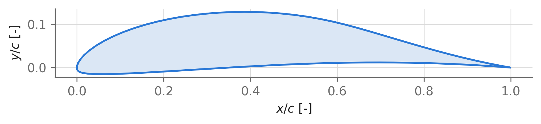
One function call gives you the complete viscous aerodynamic analysis at an operating point:
aero = af.get_aero_from_neuralfoil(
    alpha=5,   # Angle of attack [deg]
    Re=500e3,  # Chord-referenced Reynolds number [-]
    mach=0.03, # Freestream Mach number [-]
)

for key in ["analysis_confidence", "CL", "CD", "CM", "Cpmin", "Top_Xtr", "Bot_Xtr", "mach_crit"]:
    print(f"{key:20s} = {float(aero[key][0]):8.4f}")
analysis_confidence = 0.9735
CL = 1.2167
CD = 0.0102
CM = -0.1312
Cpmin = -1.5244
Top_Xtr = 0.5806
Bot_Xtr = 1.0000
mach_crit = 0.5083At this cruise-like condition the airfoil delivers \(C_L\) = 1.22 at a lift-to-drag ratio of 120. The returned dictionary actually contains 202 entries — the ones above plus boundary-layer profiles (momentum thickness \(\theta\), shape factor \(H\), and edge velocity \(u_e/V_\infty\) at stations along both surfaces). The keys you will use most:
| Key | Meaning |
|---|---|
analysis_confidence |
Probability that XFoil would reproduce this result. Above 0.9 is reliable; 0.8 if you’re feeling adventurous. |
CL, CD, CM |
Lift, drag, and quarter-chord moment coefficients. |
Cpmin |
Minimum pressure coefficient on the surface. |
Top_Xtr, Bot_Xtr |
Boundary-layer transition locations (fraction of chord), upper and lower surfaces. |
mach_crit, mach_dd |
Critical and drag-divergence Mach numbers at this \(\alpha\) and Re. |
The same call accepts the knobs you would reach for in XFoil, plus control surface deflections:
aero_flap = af.get_aero_from_neuralfoil(
    alpha=5,
    Re=500e3,
    mach=0.03,
    n_crit=9,           # Transition amplification factor (e^N method); 9 = "average wind tunnel"
    xtr_upper=1.0,      # Forced-trip location, upper surface (1.0 = free transition)
    xtr_lower=1.0,
    model_size="large", # "xxsmall" ... "xxxlarge": a speed-vs-accuracy dial
    control_surfaces=[
        asb.ControlSurface(deflection=10, hinge_point=0.75)  # 10 deg trailing-edge-down flap
    ],
)
Deflecting that plain flap adds \(\Delta C_L\) = +0.46 at fixed \(\alpha\) — computed in another fraction of a millisecond.
Two properties make this method special for design work. First, it is vectorized: pass 1D arrays for alpha, Re, and mach and the whole sweep is evaluated in one shot. Second, it is differentiable: every input, including the airfoil shape itself, can be an opti.variable(), and exact gradients flow through the network to the optimizer (Section 6.7). This is the same dual-backend trick that aerosandbox.numpy plays everywhere else in the library.
6.2 Polars: performance across \(\alpha\) and Re
An airfoil doesn’t have a polar — it has a family of them. Reynolds number changes not just the drag level but the character of the boundary layer: at \(Re = 10^4\) laminar separation dominates and the airfoil struggles; at \(Re = 10^8\) transition moves forward and the polar tightens up. Because NeuralFoil is vectorized, mapping this whole family is a one-liner: flatten a grid of operating points, evaluate, and reshape.
af = asb.Airfoil("naca4412")

alpha = np.linspace(-10, 15, 151)
Re = np.geomspace(1e4, 1e8, 5)

Alpha, Re_grid = np.meshgrid(alpha, Re)  # Vectorization needs 1D arrays: flatten, then reshape
aero = af.get_aero_from_neuralfoil(
    alpha=Alpha.flatten(),
    Re=Re_grid.flatten(),
    mach=0,
    model_size="xxxlarge",  # Most accurate model; still ~1 s for all 755 points
)
aero = {k: v.reshape(Alpha.shape) for k, v in aero.items()}
Show plotting code
import _common
import matplotlib.pyplot as plt

Re_colors = plt.cm.viridis(np.linspace(0.05, 0.85, len(Re)))

def re_label(re):
    return f"$Re = 10^{{{int(np.log10(re)):d}}}$"

fig, ax = plt.subplots(3, 1, figsize=(7, 8), sharex=True)

for i in range(len(Re)):
    ax[0].plot(alpha, aero["CL"][i, :], color=Re_colors[i])
    ax[1].plot(alpha, aero["CD"][i, :], color=Re_colors[i])
    ax[2].plot(alpha, aero["CM"][i, :], color=Re_colors[i])
    _common.label_line(
        ax[0], alpha[-1], aero["CL"][i, -1], re_label(Re[i]), Re_colors[i], dx=0.4
    )

ax[0].set_ylabel("Lift coefficient $C_L$ [-]")
ax[1].set_ylabel("Drag coefficient $C_D$ [-]")
ax[1].set_yscale("log")
ax[2].set_ylabel("Moment coefficient $C_M$ [-]")
ax[2].set_xlabel(r"Angle of attack $\alpha$ [deg]")
ax[0].set_xlim(alpha[0], alpha[-1] + 5)
plt.show()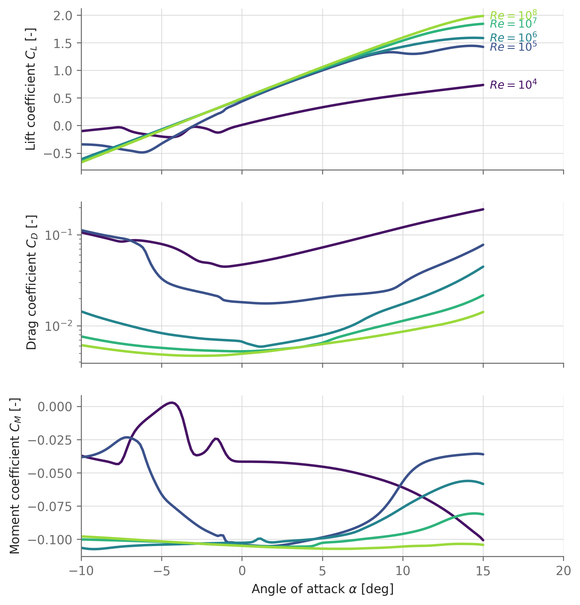
The classic way to read this data is the drag polar, \(C_L\) vs. \(C_D\). Here we also demonstrate a best practice: use analysis_confidence to visually separate results NeuralFoil is sure about from those it isn’t. At the lowest Reynolds number, parts of the polar involve delicate separation-bubble physics where even XFoil’s answers are unreliable — NeuralFoil knows this and says so.
Show plotting code
import _common
import matplotlib.pyplot as plt

def draw_airfoil_inset(ax, af, rect=(0.70, 0.05, 0.28, 0.22)):
    """Small shape reference so the polar carries its own context."""
    afax = ax.inset_axes(rect)
    afax.fill(af.x(), af.y(), facecolor="0.88", edgecolor="0.35", linewidth=1)
    afax.annotate(f"{af.name}\n", xy=(0.5, 0), ha="center", va="bottom",
                  fontsize=8, color=_common.TEXT_SECONDARY)
    afax.axis("equal")
    afax.axis("off")
    return afax

fig, ax = plt.subplots(figsize=(7, 5))

for i in range(len(Re)):
    confident = aero["analysis_confidence"][i, :] > 0.9
    CD_conf = np.where(confident, aero["CD"][i, :], np.nan)
    ax.plot(  # Low-confidence: thin and dotted
        aero["CD"][i, :], aero["CL"][i, :],
        color=Re_colors[i], linewidth=1, linestyle=":", alpha=0.6,
    )
    ax.plot(CD_conf, aero["CL"][i, :], color=Re_colors[i])
    _common.label_line(
        ax, float(aero["CD"][i, -1]), float(aero["CL"][i, -1]),
        re_label(Re[i]), Re_colors[i], dx=0.05 * float(aero["CD"][i, -1]),
    )

draw_airfoil_inset(ax, af)
ax.set_xscale("log")
ax.set_xlabel("Drag coefficient $C_D$ [-]")
ax.set_ylabel("Lift coefficient $C_L$ [-]")
plt.show()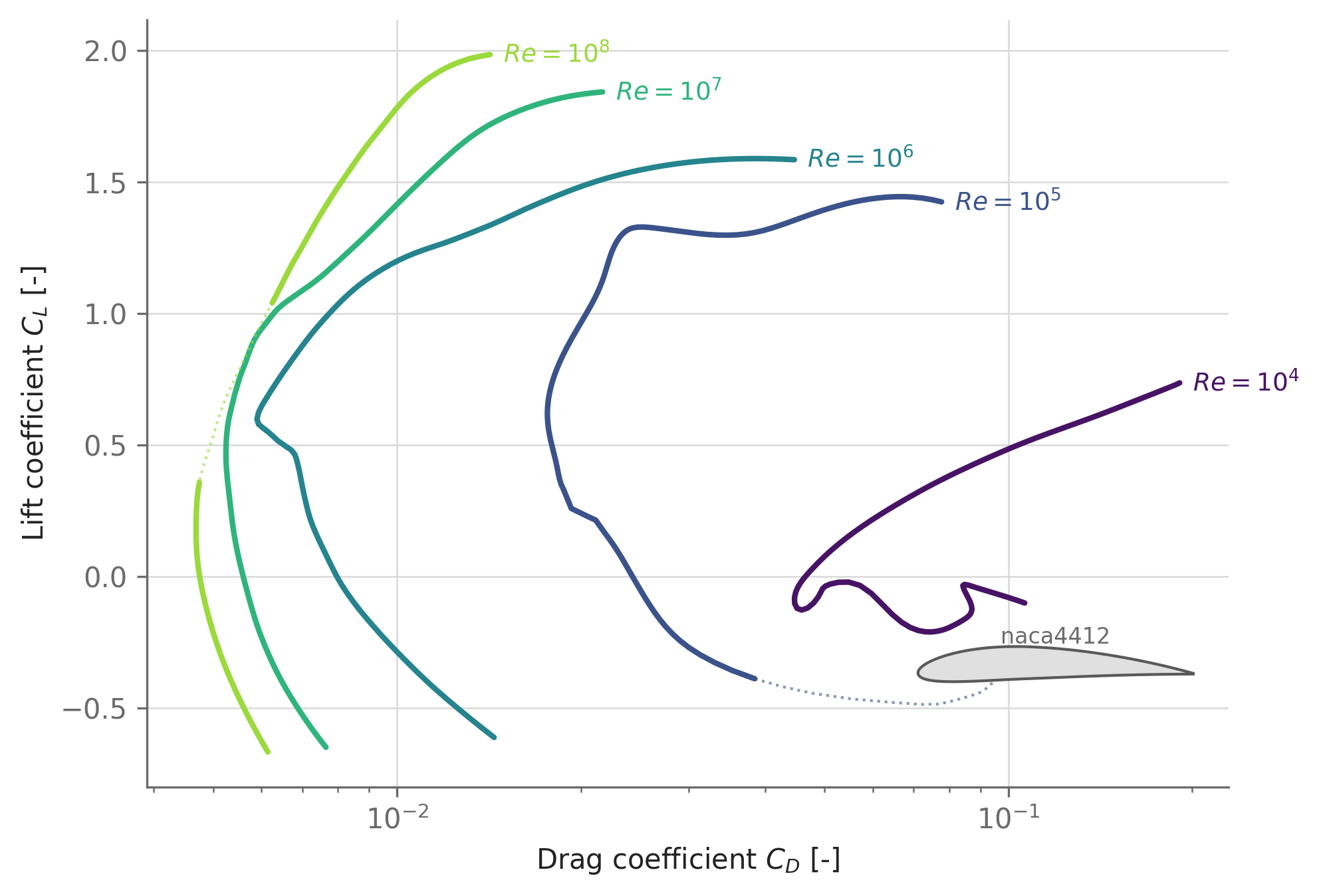
Each curve took a few milliseconds — sweeping this same grid with XFoil would take minutes and drop points wherever convergence failed. This is what makes brute-force design-space exploration (and, later, optimization) practical.
6.3 Post-stall: the full ±180° envelope
Real aircraft don’t always fly at 5° angle of attack. Propeller blades near the root, VTOL aircraft in transition, aircraft in deep stall or spin — all operate far beyond the linear range, sometimes with flow traveling backwards over the section. NeuralFoil results in AeroSandbox extend across the entire ±180° range: within roughly ±20° the neural network provides the physics, and beyond that the prediction smoothly blends into a flat-plate-theory post-stall model calibrated on wind-tunnel data.
alpha_360 = np.linspace(-180, 180, 721)
aero_360 = af.get_aero_from_neuralfoil(alpha=alpha_360, Re=1e6, mach=0)
Show plotting code
import _common
import matplotlib.pyplot as plt

fig, ax = plt.subplots(3, 1, figsize=(7, 7), sharex=True)

for a, key, label in zip(
    ax,
    ["CL", "CD", "CM"],
    ["Lift coefficient\n$C_L$ [-]", "Drag coefficient\n$C_D$ [-]", "Moment coefficient\n$C_M$ [-]"],
):
    a.plot(alpha_360, aero_360[key], color=_common.SERIES[0])
    a.set_ylabel(label)
ax[1].set_yscale("log")
ax[2].set_xlabel(r"Angle of attack $\alpha$ [deg]")
ax[2].set_xticks(np.arange(-180, 181, 45))
plt.show()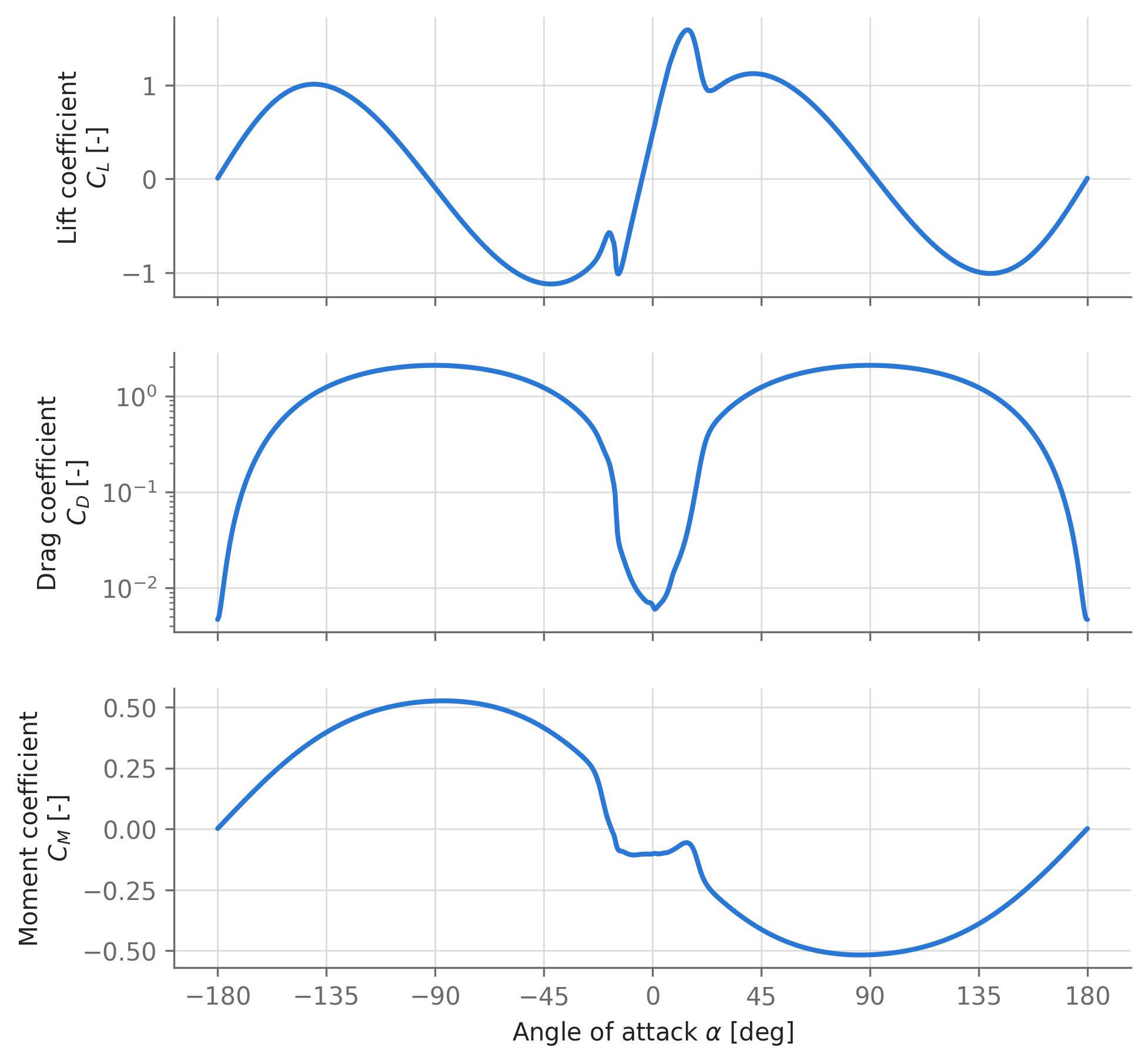
Notice the asymmetry: this cambered airfoil stalls differently at \(+15°\) than at \(-15°\), and even the reversed-flow regime (near ±180°) reflects the shape, since a sharp trailing edge makes an awkward leading edge. The 3D analysis methods in Section 7.3 rely on this 360° coverage to stay well-defined no matter where the optimizer wanders mid-solve — a key robustness property discussed in Section 3.2.
6.4 Transonic behavior and drag rise
As an airfoil approaches the speed of sound, local flow over the curved upper surface goes supersonic before the freestream does. The freestream Mach number where this first happens is the critical Mach number \(M_\mathrm{crit}\); push modestly past it and shocks appear, wave drag grows explosively, and the airfoil hits drag divergence at \(M_\mathrm{dd}\). Every NeuralFoil analysis reports both numbers, and the force coefficients include compressibility corrections, wave drag, and buffet effects.
Let’s sweep Mach number for the RAE 2822 — a classic supercritical research airfoil — and compare against three independent analysis codes of increasing fidelity, whose pre-computed results ship in the AeroSandbox repository:
rae = asb.Airfoil("rae2822")

machs = np.linspace(0.0, 1.2, 481)
aero_m = rae.get_aero_from_neuralfoil(alpha=1.0, Re=6.5e6, mach=machs)

mach_crit = float(aero_m["mach_crit"][0])  # Same at every point of the sweep:
mach_dd = float(aero_m["mach_dd"][0])      # these depend on alpha and Re, not freestream Mach
print(f"Critical Mach number:        {mach_crit:.3f}")
print(f"Drag-divergence Mach number: {mach_dd:.3f}")
Critical Mach number: 0.671
Drag-divergence Mach number: 0.739Show reference-data loading code (XFoil v6, MSES, SU2 sweeps stored in the AeroSandbox repo)
import json
from pathlib import Path

# These reference sweeps live in the AeroSandbox repository (tutorial assets).
# If you installed from PyPI they may be absent; the figure then simply omits them.
repo_root = Path(asb.__file__).parent.parent
ref_dir = (
    repo_root / "tutorial" / "06 - Aerodynamics"
    / "02 - AeroSandbox 2D Aerodynamics Tools"
    / "assets" / "RAE2822_alpha_1deg_Re_6500000"
)

def load_reference_polar(filename):
    with open(filename) as f:
        records = [json.loads(line) for line in f]
    data = {k: np.array([r[k] for r in records]) for k in records[0]}
    order = np.argsort(data["mach"])
    return {k: v[order] for k, v in data.items()}

reference_codes = {}
if ref_dir.exists():
    reference_codes = {
        "XFoil v6 (Karman-Tsien)": load_reference_polar(ref_dir / "xfoil6.csv"),
        "MSES (Euler + IBL)": load_reference_polar(ref_dir / "mses.csv"),
        "SU2 (RANS)": load_reference_polar(ref_dir / "su2.csv"),
    }
Show plotting code
import _common
import matplotlib.pyplot as plt

fig, ax = plt.subplots(figsize=(7, 5))

ref_styles = {  # color, label x-position, label y-nudge (multiplicative; log axis)
    "XFoil v6 (Karman-Tsien)": ("#999999", 0.82, 1.0),
    "MSES (Euler + IBL)": (_common.SERIES[2], 0.42, 0.68),
    "SU2 (RANS)": (_common.SERIES[3], 0.30, 1.5),
}
for label, data in reference_codes.items():
    color, x_lab, y_nudge = ref_styles[label]
    ax.plot(data["mach"], data["CD"], color=color, linewidth=1.3, alpha=0.9)
    y_lab = float(np.interp(x_lab, data["mach"], data["CD"])) * y_nudge
    ax.annotate(label, xy=(x_lab, y_lab), color=color, ha="left", va="center",
                fontsize=9, fontweight="bold")

ax.plot(machs, aero_m["CD"], color=_common.SERIES[0], zorder=4)
_common.label_line(ax, 1.03, float(np.interp(1.03, machs, aero_m["CD"])) * 1.4,
                   "ASB + NeuralFoil", _common.SERIES[0])

ax.set_yscale("log")
ax.set_ylim(2.5e-3, 0.6)
_common.annotate_event(ax, mach_crit, "$M_\\mathrm{crit}$")
_common.annotate_event(ax, mach_dd, "$M_\\mathrm{dd}$")
draw_airfoil_inset(ax, rae, rect=(0.02, 0.78, 0.28, 0.20))
ax.set_xlabel("Mach number [-]")
ax.set_ylabel("Drag coefficient $C_D$ [-]")
plt.show()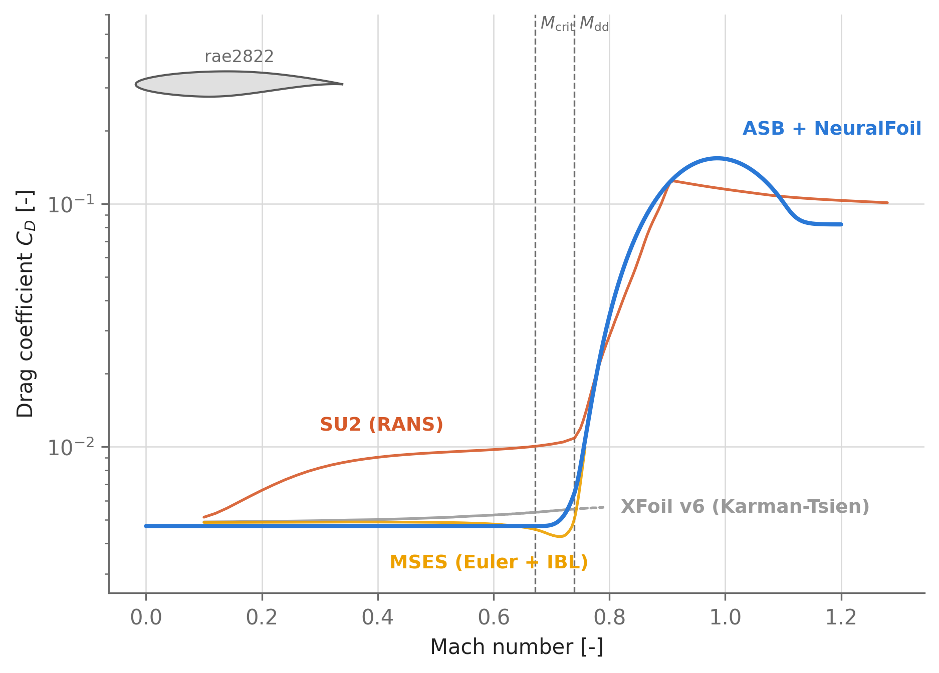
Under the hood, NeuralFoil predicts the incompressible minimum pressure coefficient, then applies a Laitone-rule compressibility correction (a higher-order cousin of Prandtl-Glauert and Karman-Tsien). Solving the corrected \(C_{p,\mathrm{min}}\) against the sonic pressure coefficient yields \(M_\mathrm{crit}\) — typically within about ±0.01 Mach of higher-fidelity codes. Past \(M_\mathrm{crit}\), empirically calibrated wave-drag and buffet models take over. The result stays smooth and differentiable across the entire range, so a transonic design optimization won’t fall off a cliff mid-solve.
Because evaluation is so cheap, you can afford to look at interactions between flow regimes that would be prohibitively expensive to map otherwise. Here is the best-achievable \(L/D\) (optimizing over \(\alpha\) at each point) across a Reynolds–Mach grid — 64,000 NeuralFoil analyses in a few seconds:
af_hale = asb.Airfoil("tasopt-c090")  # Transonic transport airfoil from MIT's TASOPT

re_g = np.geomspace(1e5, 1e7, 40)
mach_g = np.linspace(0.5, 0.9, 40)
alpha_g = np.linspace(-3, 7, 40)
Re_3, Mach_3, Alpha_3 = np.meshgrid(re_g, mach_g, alpha_g)

aero_3 = af_hale.get_aero_from_neuralfoil(
    alpha=Alpha_3.flatten(), Re=Re_3.flatten(), mach=Mach_3.flatten()
)
LD_best = np.max((aero_3["CL"] / aero_3["CD"]).reshape(Re_3.shape), axis=-1)
Show plotting code
import _common
import matplotlib.pyplot as plt

fig, ax = plt.subplots(figsize=(7, 5))
cs = ax.contourf(re_g, mach_g, LD_best, levels=15, cmap="RdBu", alpha=0.85)
cl = ax.contour(re_g, mach_g, LD_best, levels=cs.levels, colors="white", linewidths=0.5)
cbar = fig.colorbar(cs, ax=ax)
cbar.set_label(r"Best $L/D$ across $\alpha$ [-]")
ax.set_xscale("log")
draw_airfoil_inset(ax, af_hale, rect=(0.03, 0.80, 0.26, 0.18))
ax.set_xlabel("Reynolds number [-]")
ax.set_ylabel("Mach number [-]")
plt.show()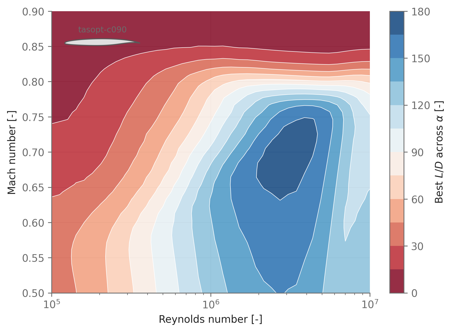
This regime — simultaneously low-Reynolds and high-Mach — is exactly where high-altitude long-endurance aircraft live, and it’s poorly covered by classical handbook data. Having a continuous model here is a genuine design capability, not just a convenience.
6.5 When to trust NeuralFoil
The honest framing: NeuralFoil is a surrogate for XFoil, so at best it reproduces XFoil’s physics — an integral-boundary-layer method that is remarkably accurate for attached and mildly separated subsonic flow over single-element airfoils. Within that envelope, NeuralFoil’s largest models match XFoil to roughly the same fidelity that XFoil matches a wind tunnel, and (as Figure 6.5 showed) its calibrated transonic extensions actually outperform XFoil v6 at high Mach. What you give up is resolution of exotic cases: multi-element airfoils, ice shapes, and hard unsteady separation are outside the training distribution.
Three practical guidelines:
- Watch
analysis_confidence. This output is a trained estimate of whether XFoil would agree with the prediction. Above 0.9, trust it; between 0.8 and 0.9, be skeptical; below that, the flow physics (or the geometry) is likely outside what any fast 2D method can handle. Constraininganalysis_confidenceduring optimization (as in Section 6.7) keeps designs inside the trustworthy region. - Pick
model_sizedeliberately. The default"large"is a good balance. Use"xxxlarge"for final polars and validation plots; drop to"medium"or smaller inside enormous optimization problems where evaluation dominates solve time. - Verify the winner. After an optimization converges, re-analyze the final design with an independent tool — XFoil, MSES, or a RANS code (Section 18.1) — before committing to it.
Speed is the reason all of this is optimization-compatible, so let’s quantify it:
import time

N = 20_000
t0 = time.perf_counter()
af.get_aero_from_neuralfoil(
    alpha=np.linspace(-10, 15, N), Re=1e6, model_size="large"
)
t_batch = time.perf_counter() - t0
throughput = N / t_batch

print(f"{N} analyses in {t_batch:.2f} s  ->  {throughput:,.0f} analyses/s "
      f"({1e6 / throughput:.0f} us per operating point)")
20000 analyses in 1.63 s -> 12,257 analyses/s (82 us per operating point)That’s 82 microseconds per viscous, compressible airfoil analysis on a single CPU — roughly four to five orders of magnitude faster than converging the same point in XFoil, and with no risk of the non-convergence holes that pepper XFoil sweeps. If you have XFoil installed, the comparison is easy to run yourself (AeroSandbox wraps it; see Section 18.1):
import shutil

if shutil.which("xfoil") is None:
    print("XFoil not found on PATH -- skipping cross-check. See the external-tools chapter.")
else:
    try:
        xfoil_aero = asb.XFoil(airfoil=af, Re=1e6, timeout=60).alpha(np.arange(0, 11, 2))
        nf_aero = af.get_aero_from_neuralfoil(
            alpha=xfoil_aero["alpha"], Re=1e6, model_size="xxxlarge"
        )
        print("alpha [deg] | CL (XFoil) | CL (NF) | CD (XFoil) | CD (NF)")
        for i, a in enumerate(xfoil_aero["alpha"]):
            print(f"{a:11.1f} | {xfoil_aero['CL'][i]:10.3f} | {nf_aero['CL'][i]:7.3f}"
                  f" | {xfoil_aero['CD'][i]:10.5f} | {nf_aero['CD'][i]:7.5f}")
    except asb.XFoil.XFoilError:
        print("XFoil is installed but crashed -- some packaged builds abort on floating-point traps.")
        print("This unreliability is, itself, part of the argument for NeuralFoil in design loops.")
XFoil is installed but crashed -- some packaged builds abort on floating-point traps.
This unreliability is, itself, part of the argument for NeuralFoil in design loops.6.6 The Kulfan parameterization: airfoils as design variables
Everything so far has been analysis: shape in, forces out. To design airfoils, we need to hand the shape itself to the optimizer — and how you parameterize the shape matters enormously. Raw coordinate arrays are a terrible choice: hundreds of variables, jagged non-smooth perturbations, and an enormous space of self-intersecting garbage between the valid designs. What we want is a basis of smooth “airfoil-like” mode shapes whose weighted sum spans realistic airfoils with a handful of numbers.
That is the Kulfan parameterization, also called CST (Class/Shape Transformation) — an industry-standard scheme, implemented in AeroSandbox as asb.KulfanAirfoil. Each surface is a class function (which hard-codes the round leading edge and sharp trailing edge that all airfoils share) multiplied by a sum of Bernstein-polynomial shape functions:
Show plotting code
import _common
import matplotlib.pyplot as plt
from math import comb

x = np.linspace(0, 1, 400)
class_function = np.sqrt(x) * (1 - x)
n = 7  # Polynomial order for 8 modes per side

fig, ax = plt.subplots(figsize=(7, 3))
mode_colors = plt.cm.viridis(np.linspace(0.05, 0.85, n + 1))
for i in range(n + 1):
    mode = class_function * comb(n, i) * x**i * (1 - x) ** (n - i)
    ax.plot(x, mode, color=mode_colors[i], linewidth=1.5)
    ax.annotate(f"{i}", xy=(x[np.argmax(mode)], np.max(mode)),
                xytext=(0, 4), textcoords="offset points",
                ha="center", color=mode_colors[i], fontsize=9, fontweight="bold")
ax.set_xlabel("$x/c$ [-]")
ax.set_ylabel("Mode shape contribution to $y/c$ [-]")
plt.show()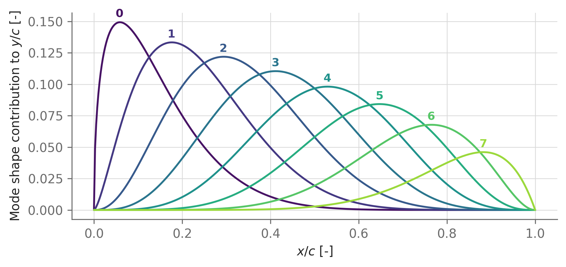
In symbols, each surface is
\[ \frac{y_\pm(x)}{c} = \underbrace{\sqrt{x}\,(1 - x)}_{\text{class function}} \; \sum_{i=0}^{7} w_{\pm,i} \underbrace{\binom{7}{i}\, x^i (1-x)^{7-i}}_{\text{Bernstein mode } i} \;+\; \frac{x\, t_\mathrm{TE}}{2}, \]
where \(w_{\pm,i}\) are the upper/lower surface weights and \(t_\mathrm{TE}\) is the trailing-edge gap thickness. AeroSandbox adds one extra leading_edge_weight mode that fine-tunes nose bluntness. Converting between representations is one method call each way:
from pprint import pprint

kulfan_af = asb.Airfoil("dae11").to_kulfan_airfoil()  # Fit Kulfan params to coordinates
pprint(kulfan_af.kulfan_parameters)
{'TE_thickness': np.float64(0.00011059192135114138),
'leading_edge_weight': np.float64(0.5035068867316296),
'lower_weights': array([-0.16310508, -0.14398528, 0.08896135, -0.0706084 , 0.09741634,
0.01466031, 0.07888292, 0.08075122]),
'upper_weights': array([0.17036014, 0.15272658, 0.51688551, 0.09212467, 0.66904449,
0.14345864, 0.28990386, 0.16207357])}Just 18 numbers describe the airfoil to visually-exact accuracy — compare that to the 81-point coordinate file it came from. KulfanAirfoil is a subclass of Airfoil, so everything you’ve seen still works: draw(), get_aero_from_neuralfoil(), and geometric queries like local_thickness(), TE_angle(), and max_camber(). Crucially, all of those are differentiable functions of the weights. You can also build one from scratch:
my_af = asb.KulfanAirfoil(
    name="My Airfoil",
    lower_weights=-0.2 * np.ones(8),
    upper_weights=+0.2 * np.ones(8),
    leading_edge_weight=0.2,
    TE_thickness=0.005,
)
That constructor is the bridge to optimization: replace those constant arrays with opti.variable() calls, and the airfoil shape becomes a set of design variables.
6.7 Airfoil shape optimization
The recipe for airfoil optimization in AeroSandbox has four steps:
- Build a
KulfanAirfoilwhose weights areopti.variable()s (initialized from a reasonable starting airfoil). - Analyze it with
get_aero_from_neuralfoil()— the outputs are now symbolic expressions of the shape. - Constrain the design to stay physical and trustworthy (“guardrails”).
- Minimize drag / maximize \(L/D\) / whatever your mission demands.
The guardrails in step 3 deserve emphasis, because optimizers are ruthless exploiters of model weaknesses (a theme this book returns to in Section 10.5). Best-practice constraints for airfoil design:
- Positive thickness everywhere (
local_thickness() > 0): rules out self-intersecting shapes, which NeuralFoil will happily “analyze” but which are geometric nonsense. - Analysis confidence (
analysis_confidence > 0.9–0.95): keeps the optimizer from wandering into regions where the aerodynamic model is unreliable — this single constraint is the difference between exploiting the physics and exploiting the surrogate. - Trailing-edge wedge angle (
TE_angle() > ~6 deg) and leading-edge weight sign constraints: manufacturability, structure, and preventing chisel-shaped noses. - Limited “wiggliness”: boundary layers respond badly to surface waviness, and wavy shapes are exactly where surrogate accuracy degrades. Borrowing the standard curvature penalty from spline smoothing, we measure wiggliness as the integrated squared second derivative of each surface, which in Kulfan-weight space is approximately
\[ w \;\approx\; \sum_{i} \left( w_{i+1} - 2 w_i + w_{i-1} \right)^2 \quad \text{(summed over both surfaces)}, \]
and constrain it to a small multiple of the starting airfoil’s value.
Here is the full recipe on a deliberately nasty problem: find the best \(L/D\) airfoil at \(Re = 5\times10^5\) and Mach 0.8 — a low-Reynolds transonic regime relevant to high-altitude aircraft, where handbook airfoils barely exist. We start from a NACA 0012, which is hopeless in this regime.
import time

Re_design = 500e3
mach_design = 0.8

initial_af = asb.KulfanAirfoil("naca0012")
opti = asb.Opti()

af_opt = asb.KulfanAirfoil(
    name="Optimized",
    lower_weights=opti.variable(init_guess=initial_af.lower_weights,
                                lower_bound=-0.5, upper_bound=0.25),
    upper_weights=opti.variable(init_guess=initial_af.upper_weights,
                                lower_bound=-0.25, upper_bound=0.5),
    leading_edge_weight=opti.variable(init_guess=initial_af.leading_edge_weight,
                                      lower_bound=-0.5, upper_bound=0.5),
    TE_thickness=0,
)
alpha_var = opti.variable(init_guess=0, lower_bound=-20, upper_bound=20)

aero_opt = af_opt.get_aero_from_neuralfoil(
    alpha=alpha_var, Re=Re_design, mach=mach_design
)

def wiggliness(af):
    return sum(
        np.sum(np.diff(np.diff(weights)) ** 2)
        for weights in [af.lower_weights, af.upper_weights]
    )

opti.subject_to([
    aero_opt["analysis_confidence"] > 0.95,        # Stay where the model is trustworthy
    af_opt.local_thickness(np.linspace(0.01, 0.99, 50)) > 0,  # No self-intersection
    af_opt.lower_weights[0] < -0.05,               # Keep a rounded (non-chisel) nose
    af_opt.upper_weights[0] > 0.05,
    af_opt.TE_angle() >= 6,                        # Manufacturable trailing edge [deg]
    wiggliness(af_opt) < 2 * wiggliness(initial_af),
])

opti.maximize(aero_opt["CL"] / aero_opt["CD"])

t0 = time.perf_counter()
sol = opti.solve(
    verbose=False,
    behavior_on_failure="return_last",  # On failure, return best iterate instead of raising
    options={
        "ipopt.mu_strategy": "monotone",     # More robust on highly non-convex problems
        "ipopt.start_with_resto": "yes",     # Prioritize feasibility from a poor start
    },
)
t_solve = time.perf_counter() - t0

af_opt = sol(af_opt)
aero_opt = sol(aero_opt)
LD_opt = float(aero_opt["CL"] / aero_opt["CD"])
print(f"Solved in {t_solve:.1f} s: L/D = {LD_opt:.1f} at alpha = {float(sol(alpha_var)):.2f} deg")
Solved in 1.7 s: L/D = 107.9 at alpha = 0.53 degShow plotting code
import _common
import matplotlib.pyplot as plt

fig, ax = plt.subplots(figsize=(7, 2.4))
ax.fill(initial_af.x(), initial_af.y(),
        facecolor="none", edgecolor="0.6", linewidth=1.2, linestyle="--")
ax.fill(af_opt.x(), af_opt.y(),
        facecolor="#dbe7f5", edgecolor=_common.SERIES[0], linewidth=1.5)
ax.set_ylim(-0.10, 0.12)
_common.label_line(ax, 0.52, 0.09, "NACA 0012 (initial guess)", "0.45", ha="center")
_common.label_line(ax, 0.52, -0.032, "Optimized", _common.SERIES[0], ha="center")
ax.set_aspect("equal")
ax.set_xlabel("$x/c$ [-]")
ax.set_ylabel("$y/c$ [-]")
plt.show()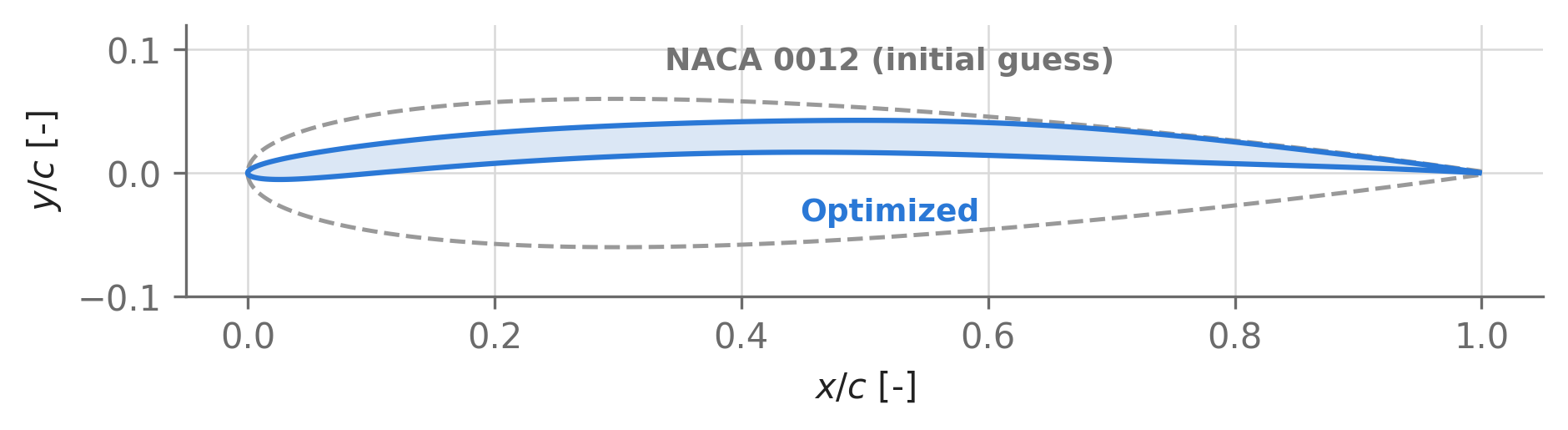
The two IPOPT options are worth remembering for airfoil work. mu_strategy: monotone trades some speed for robustness on non-convex problems, and start_with_resto: yes tells the solver to hunt for feasibility first — helpful when the initial guess (a symmetric airfoil at Mach 0.8!) is far from satisfying the constraints. behavior_on_failure="return_last" means that even if the solver stalls, you get its best iterate back for inspection instead of an exception. More on all of these in Section 5.3.
The result is textbook: the optimizer reinvents the supercritical airfoil — flattened upper surface, aft loading — from a generic starting point, in seconds, achieving \(L/D\) = 108 in a regime where the NACA 0012 starting point is nearly unflyable.
6.8 Case study: multipoint design of a human-powered-aircraft airfoil
Time for the flagship problem. In his classic paper “Pros and Cons of Airfoil Optimization” (1998), Mark Drela set up an airfoil design problem matching the MIT Daedalus human-powered aircraft: minimize drag at a lift coefficient of 1.25 and \(Re = 5\times10^5\), subject to structural and pitching-moment constraints. His central warning: single-point optimization is fraught. Ask an optimizer for the best airfoil at exactly one operating point and it will over-specialize, carving drag out at that precise \(C_L\) while performance collapses everywhere nearby. The fix is multipoint optimization: minimize a weighted average of drag across the whole realistic operating range.
We recreate Drela’s multipoint formulation here. A human-powered aircraft flies at essentially constant weight and wing area, so speed and lift coefficient are linked: flying slower raises \(C_L\) and lowers \(Re \propto V \propto C_L^{-1/2}\). Each design point therefore gets its own consistent Reynolds number:
- Objective: minimize the weighted mean of \(C_D\) over \(C_L = \{0.8, 1.0, 1.2, 1.4, 1.5, 1.6\}\), with weights \(\{5, \ldots, 10\}\) emphasizing the high-\(C_L\) (low-speed, climb-critical) end, at \(Re = 5\times10^5 \cdot (C_L / 1.25)^{-1/2}\) and \(M = 0.03\).
- Variables: the airfoil shape (17 Kulfan weights) and the angle of attack at each of the 6 operating points.
- Constraints: each point must hit its target \(C_L\); pitching moment \(C_M \geq -0.133\) everywhere (limits tail download and boom torsion); spar room \(t/c \geq 0.128\) at \(x/c = 0.33\); skin separation \(t/c \geq 0.014\) at \(x/c = 0.90\); trailing-edge angle \(\geq 6.03°\); plus the standard guardrails from Section 6.7.
CL_targets = np.array([0.8, 1.0, 1.2, 1.4, 1.5, 1.6])
CL_weights = np.array([5, 6, 7, 8, 9, 10])
Re_points = 500e3 * (CL_targets / 1.25) ** -0.5  # Constant-weight flight: Re falls as CL rises
mach_hpa = 0.03

initial_af = asb.KulfanAirfoil("naca0012")
opti = asb.Opti()

af_hpa = asb.KulfanAirfoil(
    name="NeuralFoil-optimized",
    lower_weights=opti.variable(init_guess=initial_af.lower_weights,
                                lower_bound=-0.5, upper_bound=0.25),
    upper_weights=opti.variable(init_guess=initial_af.upper_weights,
                                lower_bound=-0.25, upper_bound=0.5),
    leading_edge_weight=opti.variable(init_guess=initial_af.leading_edge_weight,
                                      lower_bound=-1, upper_bound=1),
    TE_thickness=0,
)

# One angle of attack per operating point (vector variable), initialized from thin-airfoil theory
alpha_hpa = opti.variable(
    init_guess=np.degrees(CL_targets / (2 * np.pi)), lower_bound=-5, upper_bound=18
)

aero_hpa = af_hpa.get_aero_from_neuralfoil(alpha=alpha_hpa, Re=Re_points, mach=mach_hpa)

opti.subject_to([
    aero_hpa["CL"] == CL_targets,                        # Hit every design CL
    aero_hpa["CM"] >= -0.133,                            # Pitching-moment limit, all points
    np.diff(alpha_hpa) > 0,                              # Monotonic alpha across points
    af_hpa.local_thickness(x_over_c=0.33) >= 0.128,      # Spar depth
    af_hpa.local_thickness(x_over_c=0.90) >= 0.014,      # Aft-skin separation
    af_hpa.TE_angle() >= 6.03,                           # Trailing-edge wedge angle [deg]
    # Guardrails:
    aero_hpa["analysis_confidence"] > 0.90,
    af_hpa.local_thickness() > 0,
    af_hpa.lower_weights[0] < -0.05,
    af_hpa.upper_weights[0] > 0.05,
    wiggliness(af_hpa) < 2 * wiggliness(initial_af),
])

opti.minimize(np.mean(aero_hpa["CD"] * CL_weights))

t0 = time.perf_counter()
sol = opti.solve(
    verbose=False,
    behavior_on_failure="return_last",
    options={"ipopt.mu_strategy": "monotone", "ipopt.start_with_resto": "yes"},
)
t_solve_hpa = time.perf_counter() - t0

af_hpa = sol(af_hpa)
aero_hpa = sol(aero_hpa)
assert np.max(np.abs(aero_hpa["CL"] - CL_targets)) < 1e-4  # All design points hit

print(f"Solved in {t_solve_hpa:.1f} s")
for CL_t, CD_i, a_i in zip(CL_targets, aero_hpa["CD"], sol(alpha_hpa)):
    print(f"  CL = {CL_t:.1f}:  CD = {CD_i:.5f}  (alpha = {a_i:5.2f} deg)")
Solved in 4.1 s
CL = 0.8: CD = 0.00770 (alpha = 1.21 deg)
CL = 1.0: CD = 0.00844 (alpha = 3.05 deg)
CL = 1.2: CD = 0.00951 (alpha = 4.83 deg)
CL = 1.4: CD = 0.01078 (alpha = 6.61 deg)
CL = 1.5: CD = 0.01148 (alpha = 7.54 deg)
CL = 1.6: CD = 0.01270 (alpha = 8.74 deg)How good is this, really? Drela’s paper provides two exacting benchmarks for the same requirements: the DAE-11 itself (designed by hand, by one of the world’s foremost airfoil designers) and an airfoil computationally optimized with XFoil directly in the loop via his LINDOP optimizer. Let’s compare shapes and polars against both:
Show plotting code
import _common
import matplotlib.pyplot as plt

comparison_airfoils = {
    "Initial guess (NACA 0012)": (initial_af, "0.65", "--"),
    "NeuralFoil-optimized": (af_hpa, _common.SERIES[0], "-"),
    "Expert-designed (DAE-11)": (asb.Airfoil("dae11"), _common.SERIES[3], "-"),
}
drela_dat = ref_dir.parent / "drela_opt6_90_dof.dat"  # In-repo asset; skip if absent
if drela_dat.exists():
    comparison_airfoils["XFoil/LINDOP-optimized (Drela)"] = (
        asb.Airfoil(name="Drela opt6", coordinates=str(drela_dat)),
        _common.SERIES[1], "-",
    )

fig, ax = plt.subplots(
    2, 1, figsize=(7, 7.5), gridspec_kw={"height_ratios": [1, 2.2]}
)

alpha_sweep = np.linspace(-2, 14, 161)
for name, (comp_af, color, style) in comparison_airfoils.items():
    ax[0].plot(comp_af.x(), comp_af.y(), style, color=color, linewidth=1.4,
               zorder=4 if "NeuralFoil" in name else 3)

    polar = comp_af.get_aero_from_neuralfoil(
        alpha=alpha_sweep, Re=500e3, mach=mach_hpa, model_size="xxxlarge"
    )
    ax[1].plot(polar["CD"], polar["CL"], style, color=color, linewidth=1.6,
               alpha=0.9, zorder=4 if "NeuralFoil" in name else 3, label=name)

ax[0].set_aspect("equal")
ax[0].set_xlabel("$x/c$ [-]")
ax[0].set_ylabel("$y/c$ [-]")

ax[1].axhspan(CL_targets[0], CL_targets[-1], color="0.92", zorder=0)
ax[1].annotate("multipoint\ndesign range", xy=(0.030, 0.93), fontsize=9,
               color=_common.TEXT_SECONDARY, ha="center", va="center")
ax[1].set_xlim(0, 0.04)
ax[1].set_ylim(0, 1.8)
ax[1].set_xlabel("Drag coefficient $C_D$ [-]")
ax[1].set_ylabel("Lift coefficient $C_L$ [-]")
ax[1].legend(loc="lower right", fontsize=9)
plt.show()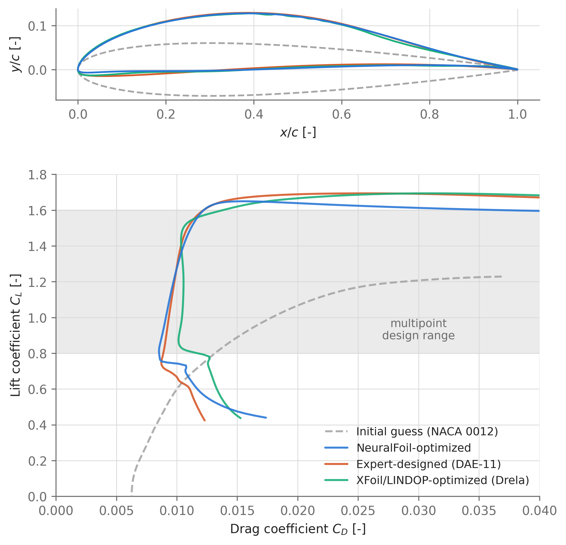
The optimizer, starting from a symmetric NACA 0012 that is comically unsuited to this mission, lands within a hair of the expert design: at the nominal \(C_L = 1.25\), our airfoil’s drag coefficient of 0.00991 sits within 0.1% of the DAE-11’s 0.00992 (both analyzed with NeuralFoil’s largest model — re-verify final candidates with an independent code per Section 6.5). Just as important, the polar stays competitive across the entire shaded design range rather than kissing the expert curve at one point — that robustness is precisely what the multipoint formulation buys, and what a single-point version of this problem would have thrown away.
The broader lesson generalizes beyond airfoils: optimize over the operating envelope you actually fly, not the single point you find easiest to write down. Multipoint objectives cost almost nothing extra here — the six operating points solved together in seconds — and they are the difference between a design that works on paper and one that works in the air.
6.9 Where to go next
- Section 7.3 lifts these 2D results into three dimensions:
AeroBuildupsweeps NeuralFoil polars across every wing cross-section to predict whole-aircraft aerodynamics. - Section 10.5 uses airfoil-level models inside wing-sizing trade studies — and expands on the “optimizers exploit weak models” lesson that motivated our guardrail constraints.
- Section 18.1 covers AeroSandbox’s interfaces to XFoil, MSES, and AVL, for independent verification of optimized designs.