Everything else in this book runs inside AeroSandbox: differentiable, vectorized, and callable as ordinary Python. But aerospace engineering has a deep bench of trusted standalone analysis codes — XFoil, AVL, and MSES from Mark Drela’s group at MIT, plus geometry-centric tools like OpenVSP and XFLR5 — and a design is more believable when an independent tool agrees with it. This chapter shows how to drive XFoil and AVL directly from AeroSandbox, how to export your geometry to OpenVSP, XFLR5, and raw AVL input files, and — just as important — the software patterns that make integrations with file-based external programs robust: guarded execution, timeouts, and defensive handling of partially-converged results.
18.1 The role of external tools
The takeaway first: external tools belong outside your optimization loop. An AeroSandbox-native analysis like NeuralFoil (Section 6.1) or AeroBuildup (Section 7.1) is a pure mathematical function — the optimizer can trace derivatives through it and evaluate thousands of design points per second. An external tool is a compiled program that communicates through files on disk: every evaluation spawns a process, writes input files, and parses text output. That makes it hundreds to thousands of times slower per point, non-differentiable, and occasionally non-convergent. Optimizing through one is possible but painful (see Section 17.4 for the escape hatch); the workflow that actually works is:
Design with AeroSandbox’s differentiable models.
Verify the optimum with an independent external tool.
If they disagree, calibrate: fit a correction to the external tool’s data (Section 17.2) and re-optimize.
This is the same “trust, but verify” discipline as Section 6.5 and Section 7.7, extended to tools that never appear inside an asb.Opti problem. AeroSandbox ships first-class interfaces to three of Drela’s codes, and exporters for several more:
One caveat up front: the runner interfaces (asb.XFoil, asb.AVL, asb.MSES) require the corresponding executable to already be on your computer — AeroSandbox does not bundle them. Download each from the linked page above and either put it on your system PATH or pass its filepath to the interface (e.g., asb.XFoil(..., xfoil_command="/path/to/xfoil")).
18.2 The guarded-execution pattern
Because the binaries may or may not exist on any given machine, code that calls them should check first and degrade gracefully. The idiom is one line with Python’s shutil.which, which searches PATH exactly like your shell does:
import aerosandbox as asbimport aerosandbox.numpy as npfrom shutil import whichxfoil_present = which("xfoil") isnotNoneavl_present = which("avl") isnotNonefor tool in ["xfoil", "avl", "mset", "mses", "mplot"]:print(f"{tool:<8}{'found'if which(tool) else'not found'}")
xfoil    found
avl      found
mset     not found
mses     not found
mplot    not found
This printout is live: it reflects the machine that rendered this book (which has XFoil and AVL installed, but not MSES). Every analysis cell in this chapter follows the same pattern —
if xfoil_present: ... # run the toolelse:print("XFoil not found -- skipping.")
— so the chapter executes cleanly on any machine, running what it can and skipping what it can’t. We recommend the same pattern for your own work whenever a script or notebook will outlive one computer: shared analysis notebooks, CI pipelines, and anything a colleague might re-run. A hard crash deep inside a subprocess call is a miserable way to learn that a cluster node doesn’t have AVL installed.
18.3 XFoil
XFoil is the reference tool for subsonic airfoil analysis — a linear-vorticity panel method coupled to a two-equation integral boundary-layer model with an \(e^N\) transition criterion. NeuralFoil (Section 6.1) was trained on XFoil data, so XFoil is the natural referee for it: fast enough to spot-check a design in seconds, and independent enough that agreement means something.
The asb.XFoil constructor takes an Airfoil and the flow condition; the analysis then runs via .alpha() (specified angle of attack) or .cl() (specified lift coefficient, letting XFoil find the angle of attack):
af = asb.Airfoil("naca2412")if xfoil_present: xf = asb.XFoil( airfoil=af, Re=1e6, # Chord-referenced Reynolds number. Re=0 (default) runs inviscid.# xfoil_command="/path/to/xfoil", # Only needed if XFoil isn't on PATH. )from pprint import pprint pprint(xf.alpha(5)) # alpha in degreeselse:print("XFoil not found -- skipping.")# Pre-captured output from a machine with XFoil 6.99, for reference:# {'CL': array([0.8099]), 'CD': array([0.00795]), 'CDp': array([0.00141]),# 'CM': array([-0.053]), 'Cpmin': array([-1.7874]), 'Chinge': array([0.0049]),# 'Top_Xtr': array([0.2938]), 'Bot_Xtr': array([0.9999]), 'alpha': array([5.])}
The result is a plain dictionary of NumPy arrays: force and moment coefficients, the minimum pressure coefficient, the hinge moment (about hinge_point_x, default \(x/c = 0.75\)), and the upper- and lower-surface transition locations. A fixed-lift analysis works the same way — useful when comparing airfoils at a common \(C_L\) rather than a common \(\alpha\):
if xfoil_present: result = xf.cl(0.8)print(f"To reach CL = 0.8: alpha = {result['alpha'][0]:.2f} deg, "f"CD = {result['CD'][0]:.5f}")else:print("XFoil not found -- skipping.")# Pre-captured: To reach CL = 0.8: alpha = 4.89 deg, CD = 0.00783
To reach CL = 0.8: alpha = 4.89 deg, CD = 0.00783
18.3.1 Sweeps, and the ragged-output rule
Both .alpha() and .cl() accept arrays and run the whole sweep in a single XFoil process, which is far faster than one process per point. But there is a critical gotcha: XFoil silently drops operating points that fail to converge, so the output arrays can be shorter than your input. Never assume positional correspondence with your requested sweep — always work from the returned "alpha" array:
if xfoil_present: result = xf.alpha([3, 5, 60]) # 60 degrees is far past stall...print(f"Requested 3 points; got {len(result['alpha'])} back.")print(f"Converged alphas: {result['alpha']}")else:print("XFoil not found -- skipping.")# Pre-captured: Requested 3 points; got 2 back. Converged alphas: [3. 5.]
For wide sweeps, .alpha() also takes a start_at argument (default 0): the sweep is internally split into two passes marching away from that anchor (e.g., 0 → +16°, then 0 → −8°), so each solution warm-starts from a well-converged neighbor. This markedly improves convergence near stall.
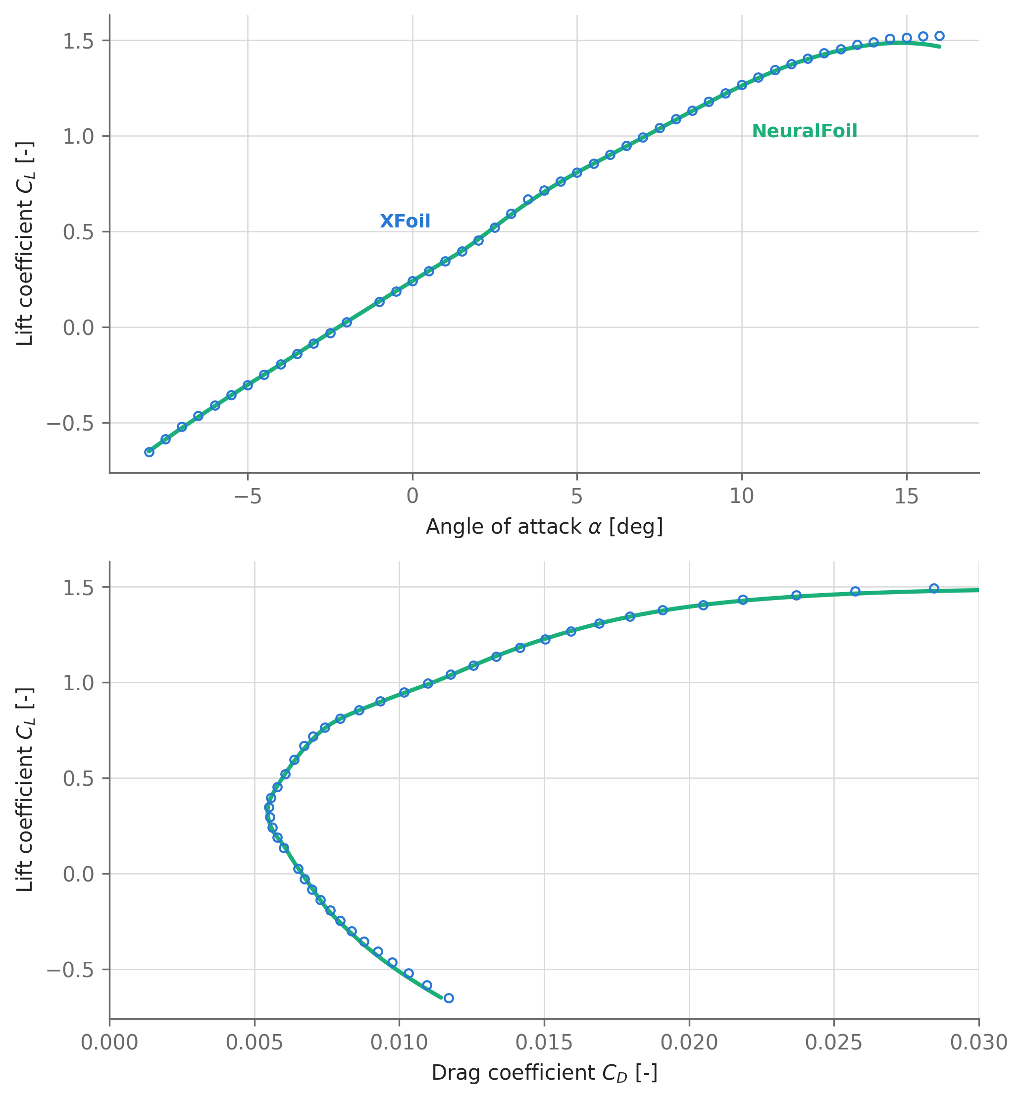
Now the payoff figure: a full polar, run live through XFoil, overlaid on NeuralFoil’s prediction for the same airfoil and Reynolds number.
Figure 18.1: NACA 2412 polar at Re = 10⁶: XFoil (points, computed live by this page) versus NeuralFoil (line). Agreement is within a few lift counts across the whole range — unsurprising, since NeuralFoil was trained on XFoil data — with the surrogate slightly smoothing the maximum-lift region. One of the 49 requested XFoil points failed to converge and was silently dropped; NeuralFoil, built to live inside optimization loops, has no such failure mode.
Converged XFoil points: 48 of 49 requested
Attached-flow (-5 to +10 deg) agreement, XFoil vs. NeuralFoil:
  max |delta CL|   = 0.0186
  mean |delta CD|  = 0.00004
Note the timeout=120 in the constructor: any single XFoil invocation — here, the whole 49-point sweep, since a sweep is one process — is killed after that many seconds (the default is 30). If a run times out, AeroSandbox issues a warning and returns whatever points converged before the kill, so a too-short timeout shows up as a mysteriously truncated polar. For very fine sweeps, set timeout=None.
18.3.2 Boundary-layer details
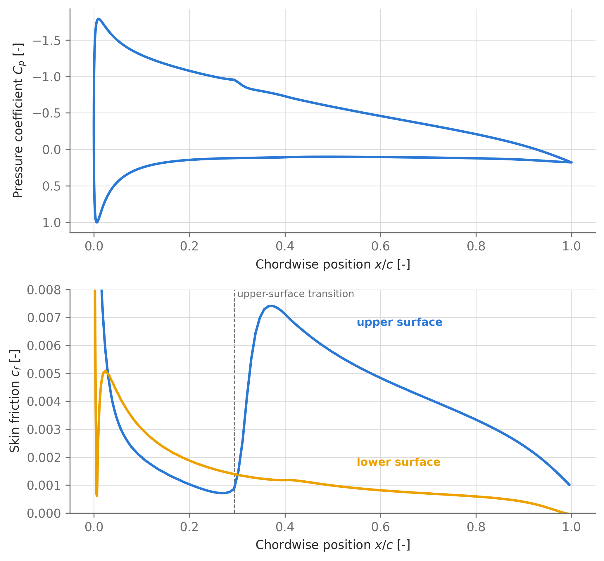
Where XFoil really earns its keep as a referee is the flow detail behind the force coefficients. Construct with include_bl_data=True and each converged point carries a pandas DataFrame of boundary-layer quantities along the surface and wake: pressure coefficient, skin friction, displacement and momentum thicknesses, and shape factor.
import _commonimport matplotlib.pyplot as pltif xfoil_present: point = asb.XFoil(airfoil=af, Re=Re, include_bl_data=True).alpha(5) bl = point["bl_data"][0] # One DataFrame per converged point surface = bl[bl["x"] <=1] # Trim the wake (x/c > 1) i_le = surface["x"].argmin() # Data runs upper TE -> LE -> lower TE upper, lower = surface.iloc[:i_le +1], surface.iloc[i_le:] fig, ax = plt.subplots(2, 1, figsize=(7, 6.5)) ax[0].plot(surface["x"], surface["Cp"], color=_common.SERIES[0]) ax[0].invert_yaxis() # Suction up, by convention ax[0].set_xlabel(r"Chordwise position $x/c$[-]") ax[0].set_ylabel(r"Pressure coefficient $C_p$[-]") ax[1].plot(upper["x"], upper["cf"], color=_common.SERIES[0]) ax[1].plot(lower["x"], lower["cf"], color=_common.SERIES[2]) ax[1].set_ylim(0, 0.008) # Clip the stagnation-point spike near the LE _common.label_line(ax[1], 0.55, 0.0068, "upper surface", _common.SERIES[0]) _common.label_line(ax[1], 0.55, 0.0018, "lower surface", _common.SERIES[2]) _common.annotate_event(ax[1], float(point["Top_Xtr"][0]),"upper-surface transition") ax[1].set_xlabel(r"Chordwise position $x/c$[-]") ax[1].set_ylabel(r"Skin friction $c_f$[-]") fig.tight_layout() plt.show()else:print("XFoil not found -- skipping the boundary-layer plot.")
Figure 18.2: XFoil boundary-layer data for the NACA 2412 at α = 5°, Re = 10⁶. Top: surface pressure distribution. Bottom: skin-friction coefficient, showing laminar flow to about 30% chord on the upper surface, the transition spike, and turbulent recovery; the lower surface stays laminar nearly to the trailing edge.
18.3.3 The knobs that matter
A few constructor arguments cover nearly all practical use:
Re, mach: the flow condition. Re=0 runs inviscid. XFoil’s compressibility handling is the Kármán–Tsien correction, which loses validity once local flow goes supersonic — for genuinely transonic work, use MSES (Section 18.5). Freestream mach >= 1 raises an error immediately.
n_crit: the \(e^N\) transition amplification factor — effectively a freestream-turbulence knob. The XFoil documentation suggests: sailplane 12–14, motorglider 11–13, clean wind tunnel 10–12, average wind tunnel 9 (the default), dirty wind tunnel 4–8.
xtr_upper, xtr_lower: forced boundary-layer trip locations in \(x/c\) (1.0, the default, means free transition). Use these to simulate trip strips, rain, or manufacturing roughness.
max_iter: viscous-solution iteration cap (default 100). Raising it rescues marginal points near stall at the cost of runtime.
working_directory: by default all file I/O happens in a throwaway temp directory; point this at a real folder to inspect the input/output files when debugging.
verbose=True: stream XFoil’s console output — the first thing to turn on when a run mysteriously fails.
18.4 AVL
AVL (Athena Vortex Lattice) is Drela and Youngren’s aircraft-level analysis code: an extended vortex-lattice model for lifting surfaces plus a slender-body model for fuselages, wrapped in a full linearized flight-dynamics analysis. Where the native VLM in Section 7.5 gives you differentiable forces for optimization, AVL’s specialty is the stability picture: a complete set of static and dynamic derivatives, control derivatives, and the neutral point, all from one run.
asb.AVL translates an asb.Airplane directly into AVL’s input format — no hand-written .avl files. To show it working, we reuse the same glider as Section 7.2, which lets us cross-check AVL against the native analyses of that chapter:
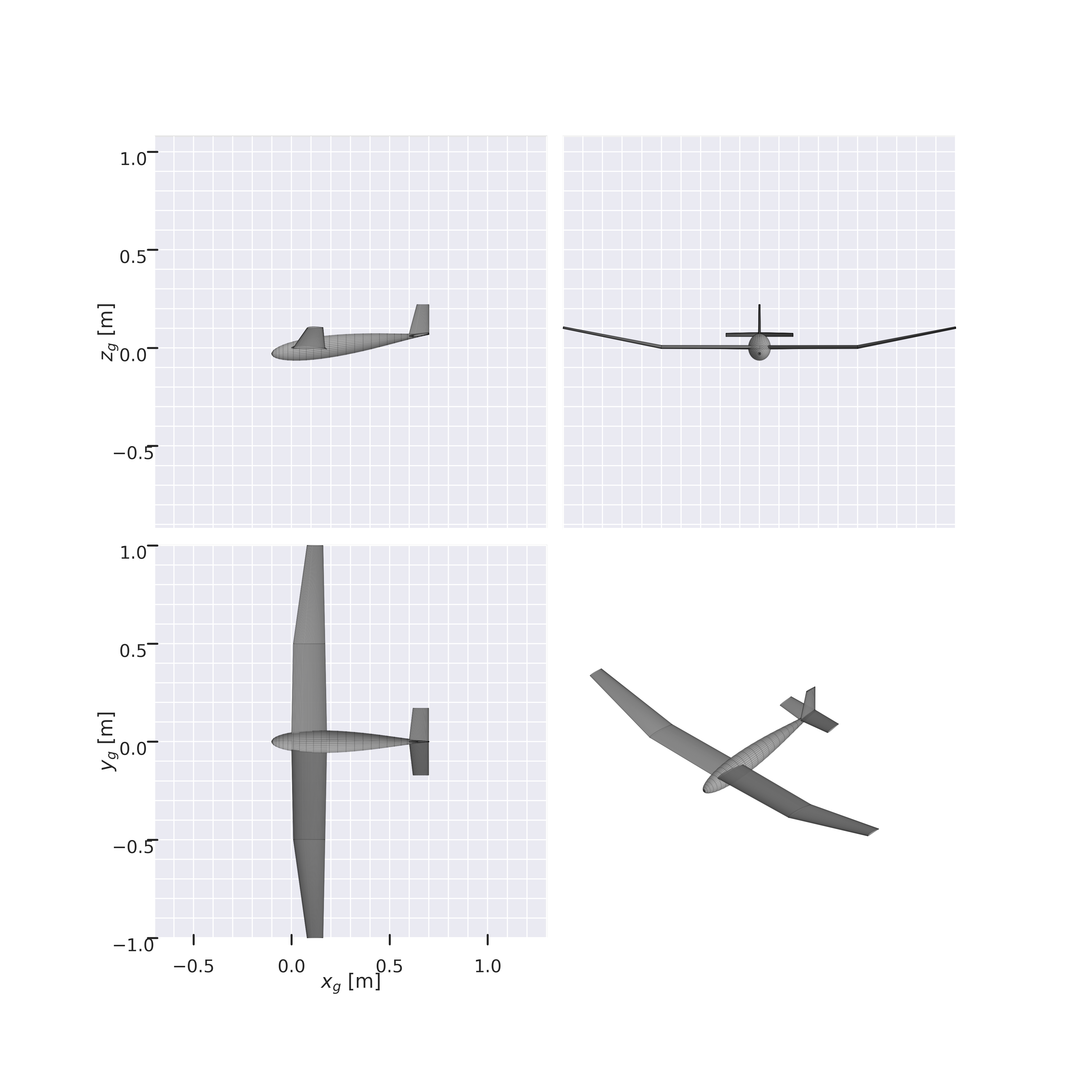
Peter’s Glider — the same geometry as the aircraft-aerodynamics chapter
<module '_common' from '/tmp/claude-1000/-home-psharpe-gh-AeroSandbox/1ccf6b40-3256-4f8d-9484-ebe00c7e55db/scratchpad/book-staging/_common.py'>
18.4.1 What gets sent to AVL
Before running anything, it’s worth seeing what AeroSandbox writes, because this is the pattern every file-based interface follows. write_avl() generates the complete AVL input deck — and it needs no AVL binary at all, so it always runs:
import tempfilefrom pathlib import Pathop_point = asb.OperatingPoint( velocity=25, # m/s alpha=3, # deg)avl = asb.AVL(airplane=airplane, op_point=op_point)case_dir = Path(tempfile.mkdtemp())avl.write_avl(case_dir /"glider.avl")print("Files written:", *sorted(p.name for p in case_dir.iterdir()), sep="\n ")print("\nHead of glider.avl:\n")print("\n".join((case_dir /"glider.avl").read_text().splitlines()[:16]))
Files written:
  glider.avl
  glider.avl.af0
  glider.avl.af1
  glider.avl.af2
  glider.avl.af3
  glider.avl.af4
  glider.avl.af5
  glider.avl.af6
  glider.avl.fuse0

Head of glider.avl:

Peter's Glider
#Mach
0        ! AeroSandbox note: This is overwritten later to match the current OperatingPoint Mach during the AVL run.
#IYsym   IZsym   Zsym
0       0   0
#Sref    Cref    Bref
0.29237742155477453 0.1510464169994095 2.019809790962264
#Xref    Yref    Zref
0 0 0
# CDp
0
#===============================================================================
SURFACE
Main Wing
#Nchordwise  Cspace  [Nspanwise   Sspace]
12   1   12   1
One .avl file holds the surface layout, and sidecar files carry each cross-section’s airfoil coordinates (.af0, .af1, …) and the fuselage profile (.fuse0). Control surfaces declared on WingXSecs are written as AVL CONTROL cards automatically. This is also your escape hatch: if you want AVL features AeroSandbox doesn’t wrap (eigenmode analysis, trim calculations, mass files), export the deck and drive AVL by hand from here.
18.4.2 Running it
.run() executes AVL and parses everything it reports back — one call, roughly eighty outputs:
if avl_present: aero = avl.run()print(f"AVL returned {len(aero)} outputs. A selection:\n")for group, keys in {"Forces/moments": ["CL", "CD", "Cm"],"Longitudinal ": ["CLa", "Cma", "Cmq", "Xnp"],"Lateral ": ["CYb", "Clb", "Cnb", "Clp", "Cnr"],"Span efficiency": ["e"], }.items():print(f" {group}: "+", ".join(f"{k} = {aero[k]:.4g}"for k in keys))else:print("AVL not found -- skipping.")# Pre-captured output from a machine with AVL 3.36, for reference:# Forces/moments : CL = 0.5835, CD = 0.01283, Cm = -0.06524# Longitudinal : CLa = 6.461, Cma = -2.808, Cmq = -17.32, Xnp = 0.06565# Lateral : CYb = -0.1667, Clb = -0.1654, Cnb = 0.009494,# Clp = -0.6169, Cnr = -0.02043# Span efficiency: e = 0.6737
Rate derivatives (p, q, r) are taken in body axes, matching the AeroSandbox convention for OperatingPoint (this is set automatically in the run script — plain AVL defaults to stability axes for some outputs).
Xnp is the neutral point’s \(x\) location in geometry axes; the static margin follows as (Xnp - x_cg) / c_ref.
Moments are referenced about xyz_ref (taken from the Airplane unless you override it in the asb.AVL constructor).
Alongside the coefficients, AeroSandbox adds dimensional conveniences: forces in Newtons resolved in body, wind, and geometry axes (F_b, F_w, F_g), and likewise for moments.
18.4.3 Cross-checking AVL against the native stack
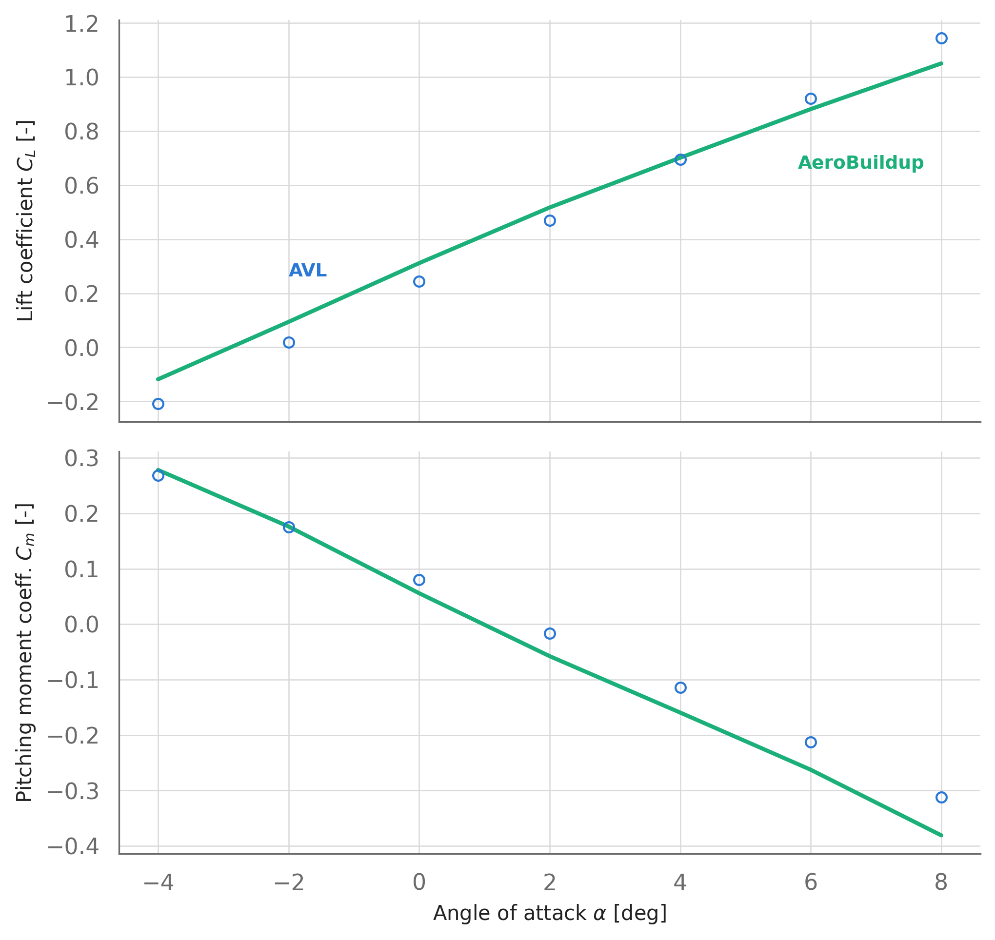
Because this is the same airplane as Section 7.2, we can do exactly what this chapter preaches: use the external tool as a referee. The loop below runs AVL at several angles of attack — note that unlike the vectorized native analyses, each point is a separate subprocess — and overlays asb.AeroBuildup:
import _commonimport matplotlib.pyplot as pltalphas = np.arange(-4, 9, 2)aero_ab = asb.AeroBuildup( airplane=airplane, op_point=asb.OperatingPoint(velocity=25, alpha=alphas), # vectorized).run()if avl_present: aero_avl = [ asb.AVL( airplane=airplane, op_point=asb.OperatingPoint(velocity=25, alpha=alpha), ).run()for alpha in alphas # one subprocess per point ] fig, ax = plt.subplots(2, 1, figsize=(7, 6.5), sharex=True) ax[0].plot(alphas, aero_ab["CL"], color=_common.SERIES[1]) ax[0].plot(alphas, [a["CL"] for a in aero_avl], "o", color=_common.SERIES[0], markersize=5, markerfacecolor="none") _common.label_line(ax[0], 5.8, 0.68, "AeroBuildup", _common.SERIES[1]) _common.label_line(ax[0], -2.0, 0.28, "AVL", _common.SERIES[0]) ax[0].set_ylabel(r"Lift coefficient $C_L$[-]") ax[1].plot(alphas, aero_ab["Cm"], color=_common.SERIES[1]) ax[1].plot(alphas, [a["Cm"] for a in aero_avl], "o", color=_common.SERIES[0], markersize=5, markerfacecolor="none") ax[1].set_xlabel(r"Angle of attack $\alpha$[deg]") ax[1].set_ylabel(r"Pitching moment coeff.$C_m$[-]") fig.tight_layout() plt.show()else:print("AVL not found -- skipping the comparison sweep.")
Figure 18.4: Lift and pitching moment versus angle of attack for the glider: AVL (points, computed live) against the native AeroBuildup analysis (line). Two independent methods — a vortex lattice and a buildup of NeuralFoil section data — tell the same story about lift-curve slope and pitch stiffness.
This is the healthiest possible relationship with an external tool: seven subprocess calls, run occasionally as a referee — not ten thousand calls inside an optimization loop.
18.4.4 Control surfaces and analysis options
Control-surface deflections set on the geometry flow straight through — deflect the elevator, rerun, and watch the pitching moment respond:
elevator = airplane.wings[1].xsecs[0].control_surfaces[0]if avl_present:print("elevator [deg] Cm [-]")for deflection in [-10, 0, 10]: elevator.deflection = deflection # trailing-edge-down positive aero_deflected = asb.AVL(airplane=airplane, op_point=op_point).run()print(f"{deflection:14}{aero_deflected['Cm']:9.4f}")else:print("AVL not found -- skipping.")# Pre-captured: elevator [deg] Cm [-]# -10 0.1210# 0 -0.0652# 10 -0.2503elevator.deflection =0# Reset for the cells below
elevator [deg]    Cm [-]
           -10    0.1210
             0   -0.0652
            10   -0.2503
Tool-specific numerical settings — panel counts, spacing distributions, profile-drag adders — ride along on the geometry itself through the analysis_specific_options mechanism, keyed by analysis class. This keeps the Airplane definition tool-agnostic while still letting each tool be tuned:
airplane.wings[0].analysis_specific_options[asb.AVL] =dict( spanwise_resolution=24, # default is 12)### Proof, straight from the regenerated input deck (main wing SURFACE header):deck = asb.AVL(airplane=airplane, op_point=op_point).write_avl()lines = deck.splitlines()i = lines.index("Main Wing")print("\n".join(lines[i : i +3]))
Main Wing
#Nchordwise  Cspace  [Nspanwise   Sspace]
12   1   24   1
Other AVL-specific constructor options worth knowing: ground_effect=True mirrors the airplane about a ground plane (for takeoff/landing analysis), and timeout (default 5 seconds — AVL runs are fast, so a hang almost always means a malformed input deck, not a slow solve).
18.5 MSES
MSES is Drela’s transonic airfoil suite: a streamline-curvature Euler solver coupled to the same integral boundary-layer machinery as XFoil. Reach for it when XFoil’s physics run out — shocked transonic flow past \(M_\mathrm{crit}\) — or for multi-element airfoil systems. It is actually three programs (mset grids, mses solves, mplot extracts results), and AeroSandbox orchestrates all three behind a single call:
mses_present =all(which(cmd) for cmd in ["mset", "mses", "mplot"])if mses_present: ms = asb.MSES(airfoil=asb.Airfoil("rae2822")) result = ms.run( alpha=1, Re=6.5e6, mach=np.linspace(0.60, 0.78, 7), # inputs broadcast against each other )print({k: v for k, v in result.items() if k in ["mach", "CL", "CD"]})else:print("MSES executables not found on PATH -- skipping this analysis.")
MSES executables not found on PATH -- skipping this analysis.
The interface mirrors asb.XFoil — run() broadcasts alpha, Re, and mach against each other, drops unconverged points, and returns a dictionary of arrays — plus a few MSES-specific practicalities:
Distribution: unlike XFoil and AVL, MSES is not a public download; academics can obtain it through the MIT Technology Licensing Office.
X11: the MSES programs open X11 windows even in batch use. On headless machines (CI boxes, WSL, clusters), install Xvfb and AeroSandbox will automatically detect and use it as a virtual display; without X11 or Xvfb, runs fail at the mset step.
Timeouts are per-program: timeout_mset, timeout_mses (default 60 s — transonic cases genuinely take a while), and timeout_mplot.
behavior_after_unconverged_run chooses whether a mid-sweep failure re-initializes the flow solution and continues ("reinitialize", default) or abandons the rest of the sweep ("terminate").
18.6 Exporting geometry to other tools
Sometimes you don’t want AeroSandbox to run anything — you want to hand the design to another tool or teammate. Every asb.Airplane exports itself; none of these require the target program to be installed:
export_dir = Path(tempfile.mkdtemp())### AVL input deck (same writer that asb.AVL uses internally):airplane.export_AVL(export_dir /"glider.avl")### XFLR5 XML (import in XFLR5 via File -> Import -> Import from XML):airplane.export_XFLR5_xml( export_dir /"glider.xml", mass_props=asb.MassProperties(mass=1.2, x_cg=0.05), # XFLR5 wants inertia mainwing=airplane.wings[0], elevator=airplane.wings[1], fin=airplane.wings[2],)### OpenVSP script (run in OpenVSP via File -> Run Script...):vspscript = airplane.export_OpenVSP_vspscript(export_dir /"glider.vspscript")print("Exported:", *sorted(p.name for p in export_dir.iterdir()), sep="\n ")print("\nHead of glider.vspscript:\n")print("\n".join(vspscript.splitlines()[:5]))
Exported:
  glider.avl
  glider.avl.af0
  glider.avl.af1
  glider.avl.af2
  glider.avl.af3
  glider.avl.af4
  glider.avl.af5
  glider.avl.af6
  glider.avl.fuse0
  glider.vspscript
  glider.xml

Head of glider.vspscript:

// This *.vspscript file was automatically generated by AeroSandbox 4.2.9
// using syntax tested on OpenVSP 3.36.0.
// To run this script, open OpenVSP and go to File -> Run Script...

void main()
The OpenVSP path is a .vspscript file — a program in OpenVSP’s scripting language that rebuilds your wings, fuselages, and propulsors as native, editable OpenVSP geometry (not a dead mesh import). From OpenVSP you can then reach its own ecosystem: VSPAERO, structured meshing, CFD pre-processing, and photorealistic renders. For CAD workflows, Airplane.export_cadquery_geometry() writes a STEP file via CadQuery.
18.7 File-based interfaces: patterns and gotchas
All three runner interfaces share one architecture, and knowing it makes every failure debuggable. Each call:
creates a temporary working directory (override with working_directory= to keep the files);
launches the executable as a subprocess and types into its interactive text menus via stdin (there is no API; these are 1980s–90s Fortran programs, and that is precisely why they’re still trusted);
enforces a timeout, killing the process if it wedges;
parses the text output files into a plain dictionary of floats and arrays.
When something goes wrong, work that list in reverse. The debugging toolkit, in the order to try it:
verbose=True — stream the tool’s own console output. Convergence stalls, geometry complaints, and menu mis-navigation all show up here first.
working_directory="some/local/folder" — keep the input and output files, then run the tool by hand on those exact inputs to reproduce the problem outside Python.
timeout=None — rule out the watchdog. Remember the timeout covers a whole sweep in one process (XFoil) and that partial, warning-accompanied results are returned after a timeout kill — a truncated polar usually means a too-tight timeout, not bad aerodynamics.
open_interactive() (Windows) — pops the tool open in a console window, with your geometry pre-loaded, for manual exploration.
Beyond that, three gotchas account for most real-world grief:
Ragged outputs. Unconverged points are silently dropped (XFoil, MSES). Downstream code must join on the returned "alpha" (or "mach") values, never on input position. This is the single most common external-tool bug we see.
Binary provenance. “XFoil” is not one program: builds of nominally the same version differ in compiler flags and output formats, and AeroSandbox’s parsers target Mark Drela’s official distributions. Two concrete failure modes we have verified: some Linux distribution packages (e.g., the Debian/Ubuntu aptxfoil package) are compiled with floating-point-exception trapping enabled and crash outright on routine viscous cases; and other rebuilds emit polar files with extra or missing columns, which surfaces in AeroSandbox as an XFoilError: ... output file is malformed, with the raw file printed for inspection. If you hit either, suspect your binary before your geometry: swap in a known-good build (Drela’s official binaries, where available for your platform) and re-run. Even self-compiled builds from the official source can drift — we have seen output-format differences between nominally identical versions.
Don’t put them in the loop. No derivatives flow through a subprocess, so an external tool can’t sit inside an asb.Opti model directly. If you truly must optimize on one, asb.black_box wraps arbitrary functions with finite-difference gradients (Section 17.4) — but convergence noise from the tool becomes gradient noise for the optimizer, and each gradient costs one run per input dimension. The pattern that works better in almost every case: sample the external tool offline over your design region, fit or interpolate a differentiable surrogate (Section 17.2), optimize on that, and verify the optimum with the real tool — closing the loop at human timescale, not optimizer timescale.
18.8 Where to go next
Section 6.5 develops the “when to trust NeuralFoil vs. XFoil” question quantitatively, from the 2D side.
Section 7.7 does what this chapter recommends at aircraft level: four analysis methods, one wind-tunnel dataset, and an honest accounting of who was right.
Section 17.4 covers the machinery for wrapping non-differentiable functions — external tools included — when you really do need them inside an optimization problem.