import aerosandbox as asb
import aerosandbox.numpy as np

L = 10.0   # Beam length [m]
E = 228e9  # Elastic modulus [Pa] (unidirectional carbon fiber, typical)
I = 1e-6   # Area moment of inertia of the cross-section [m^4]
q = 100.0  # Uniform distributed load, pointing up [N/m]

opti = asb.Opti()

y = np.linspace(0, L, 50)  # Discretize the beam at 50 stations [m]

u = opti.variable(init_guess=np.zeros_like(y))  # Vertical deflection [m]
du = opti.derivative_of(u, with_respect_to=y, derivative_init_guess=0)
ddu = opti.derivative_of(du, with_respect_to=y, derivative_init_guess=0)
dddu = opti.derivative_of(ddu, with_respect_to=y, derivative_init_guess=0)

opti.constrain_derivative(  # The governing equation: E I u'''' = q
    variable=dddu,
    with_respect_to=y,
    derivative=q / (E * I),
)

opti.subject_to([
    u[0] == 0,      # Cantilever root: no deflection...
    du[0] == 0,     # ...and no slope.
    ddu[-1] == 0,   # Free tip: no bending moment...
    dddu[-1] == 0,  # ...and no shear.
])

sol = opti.solve(verbose=False)9 Structures
This chapter shows how to size aircraft structure from physics, inside the same optimization problem as everything else. You’ll learn to solve Euler–Bernoulli beam bending directly with asb.Opti, to size a minimum-mass composite wing spar with TubeSparBendingStructure, to guard a design against buckling with the checks in aerosandbox.structures.buckling, and finally to distill a physics model into a reusable scaling law — the same process that produced the structural mass models in aerosandbox.library. This matters because structural weight is the counterweight to nearly every aerodynamic desire: span, aspect ratio, and load factor are all cheap until the structure has to pay for them. The fidelity of your structural model largely determines where the optimizer pushes your design (see Section 10.5 for what happens when it pushes back too weakly).
9.1 Why physics-based structures?
There are two broad ways to estimate structural mass in conceptual design. Statistical weight models (regressions over historical aircraft, covered in Section 9.4) are excellent when your design lives inside the data cloud they were fit to — and quietly wrong when it doesn’t. Physics-based models compute loads and stresses from first principles, so they extrapolate to unconventional configurations: very high aspect ratios, multi-boom layouts, unusual load cases.
For wings, physics-based modeling is unusually affordable. A high-aspect-ratio wing’s primary structure is, to a good approximation, a cantilever beam — long, slender, loaded mostly in bending. Classical beam theory captures the dominant physics, and a discretized beam solves in milliseconds. That’s cheap enough to embed inside the design optimization rather than run as a separate analysis.
The embedding uses the same trick as trajectory optimization (Section 12.1): pose the discretized governing differential equation as a set of equality constraints, and let the optimizer converge the physics and the design simultaneously. In the MDO literature this is called simultaneous analysis and design (SAND). There is no inner FEA loop to converge on every function evaluation — the beam equation is only exactly satisfied at the optimum, which is the only place you needed it to be.
9.2 Beam bending as an optimization problem
Start with the simplest structural member on an airplane: a cantilever. Think of one half of a wing, clamped at the fuselage centerline and free at the tip. A distributed aerodynamic load pushes up along its length; the beam bows upward; the material near the root works hardest, because every newton of lift outboard acts through a long moment arm.
Euler–Bernoulli beam theory turns this picture into a fourth-order ordinary differential equation for the vertical deflection \(u(y)\):
\[ \frac{\mathrm{d}^2}{\mathrm{d}y^2}\left(E I \, \frac{\mathrm{d}^2 u}{\mathrm{d}y^2}\right) = q(y) \tag{9.1}\]
where \(y\) is the distance along the beam, \(E\) is the material’s elastic modulus, \(I\) is the cross-section’s area moment of inertia (so \(EI\) is the bending stiffness), and \(q(y)\) is the applied force per unit length. Four boundary conditions close the problem: at a cantilever root, deflection and slope are zero; at a free tip, bending moment (\(EI\,u''\)) and shear (\((EI\,u'')'\)) are zero.
To solve this in AeroSandbox, we discretize the beam at \(N\) stations and rewrite the fourth-order ODE as a chain of first-order relationships, each enforced by trapezoidal collocation via opti.derivative_of() and opti.constrain_derivative() — exactly the machinery used for trajectory dynamics in Section 12.1:
Notice what’s missing: there is no opti.minimize() call. With the geometry fixed, the beam equation plus boundary conditions has exactly one solution, so this is a feasibility problem — simulation posed as optimization, with zero design freedom (see Section 5.6). IPOPT solves it in a handful of iterations.
For a uniformly-loaded cantilever, the exact solution is known, so we can check ourselves:
\[ u(y) = \frac{q \, y^2}{24\,EI}\left(6L^2 - 4Ly + y^2\right), \qquad u_\mathrm{tip} = \frac{q L^4}{8\,EI} \]
u_num = sol(u)
u_analytic = q * y**2 * (6 * L**2 - 4 * L * y + y**2) / (24 * E * I)
The collocated solution gives a tip deflection of 0.5482 m against an analytic value of 0.5482 m — a worst-case error along the beam of 0.04 mm, or 0.007% of the tip deflection, with just 50 points (Figure 9.1). Trapezoidal collocation converges at second order, so doubling the grid buys roughly a 4\(\times\) error reduction — though for sizing work, this is already far below the uncertainty in your loads.
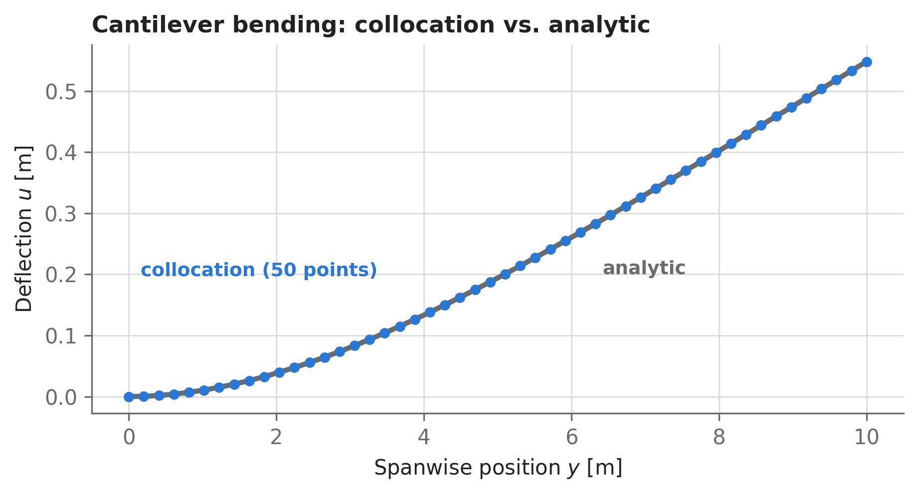
asb.Opti, reproduces the analytic Euler–Bernoulli solution.
This from-scratch pattern is worth knowing because it generalizes: nonuniform stiffness, added torsion, coupled aerodynamic loads (Chapter 14) — all are just more variables and more constraints in the same Opti problem. But for the most common case, a cantilevered tube spar, AeroSandbox packages the whole thing.
9.3 Sizing a tube spar
Here is the motivating case for the rest of the chapter, borrowed from human-powered-aircraft practice (think MIT’s Daedalus): a 34-meter-span airplane with a gross mass of 104 kg, whose wing is held up by a single circular carbon-fiber tube spar. The tube’s diameter is fixed at 3.5 inches (89 mm, measured to the wall centerline) — say, by the mandrel your shop owns — but the wall thickness can vary freely along the span, so the question is: how should material be distributed to carry the design load at minimum mass?
TubeSparBendingStructure (in aerosandbox.structures) builds exactly this problem. It is an ImplicitAnalysis: you hand it your Opti instance, and it adds its own state variables (the deflection chain from Section 9.2) and physics constraints to your problem. Geometry parameters can be numbers, functions of span, or None — where None means “make this a design variable at every station.” For a thin-walled tube of mean diameter \(d\) and wall thickness \(t\), it uses \(I = \frac{\pi}{8} d^3 t\), and it reports the extreme-fiber axial stress \(\sigma(y) = E \, u''(y) \, d_\mathrm{outer}/2\) at every station.
We size the structure at the ultimate load case: level-flight lift scaled by an ultimate load factor \(n_\mathrm{ult} = 1.75\) (the Daedalus design value), distributed elliptically over the span. Two constraints bound the design from below: an allowable stress of 500 MPa (a conservative working value for unidirectional carbon, with knockdowns for joints and fatigue baked in), and a minimum manufacturable wall gauge of 0.2 mm.
import aerosandbox.tools.units as u  # Unit conversion constants (all to SI)
from aerosandbox.structures.tube_spar_bending import TubeSparBendingStructure

span = 34.0        # Total wingspan [m]
mass_total = 104.0 # Gross mass the wing must lift [kg]
n_ult = 1.75       # Ultimate load factor [-]
E = 228e9          # Elastic modulus, unidirectional carbon [Pa]
rho = 1600.0       # Density of carbon laminate [kg/m^3]
stress_allowable = 500e6  # Allowable axial stress [Pa]

half_span = span / 2
lift = n_ult * mass_total * 9.81  # Total lift at the ultimate load case [N]


def elliptical_lift_distribution(y):
    """Lift per unit span [N/m] at spanwise station y [m]."""
    return (lift / span) * (4 / np.pi) * (1 - (y / half_span) ** 2) ** 0.5


def make_spar_problem():
    opti = asb.Opti()
    beam = TubeSparBendingStructure(
        opti=opti,
        length=half_span,
        diameter_function=3.5 * u.inch,  # Fixed diameter along the whole spar [m]
        wall_thickness_function=None,    # None -> free design variable at each station
        points_per_point_load=50,
        bending_distributed_force_function=elliptical_lift_distribution,
        elastic_modulus_function=E,
    )
    opti.subject_to([
        beam.stress_axial <= stress_allowable,
        beam.wall_thickness >= 0.2e-3,  # Minimum manufacturable gauge [m]
    ])
    spar_mass = 2 * beam.volume() * rho  # Both wing halves [kg]
    opti.minimize(spar_mass)
    return opti, beam, spar_mass


opti, beam, spar_mass = make_spar_problem()
sol = opti.solve(verbose=False)

beam_a = sol(beam)  # Substituting the solution gives a numeric copy of the analysis
mass_a = sol(spar_mass)
The optimized spar weighs 10.21 kg for both wing halves — about 10% of gross mass. Figure 9.2 shows where that mass went. (For a quick interactive look at any solved beam, beam_a.draw() produces a similar diagnostic plot.)
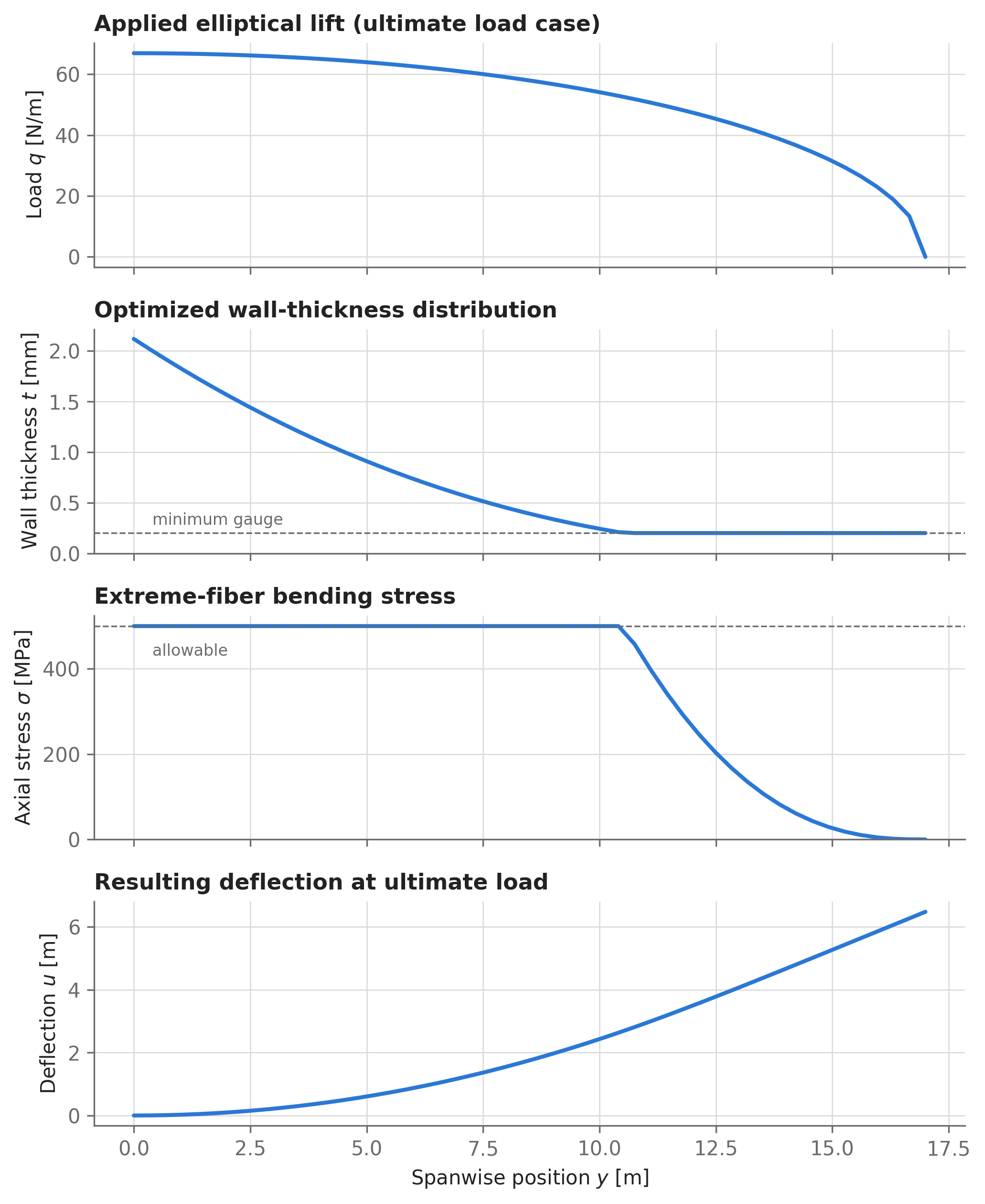
Read the middle two panels together and you can see the optimizer’s logic. Over the inboard span, the stress constraint is active everywhere: the wall thins in perfect proportion to the falling bending moment so that the material always works at exactly 500 MPa. This is the classic fully-stressed design, and here it emerges from the optimizer rather than being assumed. Outboard of roughly 10 m, the 0.2 mm gauge floor becomes the binding constraint instead, and stress drops below the allowable — the material there exists because you can’t roll a thinner tube, not because the loads demand it.
NoteSimplifications in this model
This is a conceptual-sizing model, and it leaves things out deliberately: no relief from the wing’s own weight (conservative), a single symmetric pull-up load case, no torsion or sweep effects, no joint/fitting mass, and a thin-wall approximation for the tube (error \(\sim (t/d)^2\), well under 1% here). The point of a physics-based model is that each of these is a visible, removable assumption — not an artifact buried in a regression.
9.3.1 The failure mode we forgot
Step on an empty soda can: long before the aluminum itself crushes, the thin wall wrinkles and collapses. Thin-walled tubes in compression fail the same way — a local instability called crippling — and the compression side of a bent spar is loaded exactly like that can. The classical design allowable (Raymer eq. 14.33, also in the Air Force Stress Manual) is
\[ \sigma_\mathrm{crippling} = 0.3 \, \frac{E\,t}{r} \]
which shrinks as the wall gets thinner relative to the tube radius. Our optimizer just spent its whole effort making walls thin. Did it walk into this failure mode? Let’s check, using aerosandbox.structures.buckling:
from aerosandbox.structures.buckling import (
    thin_walled_tube_crippling_buckling_critical_load,
)


def crippling_allowable_stress(beam):
    """Compressive stress [Pa] at which the tube wall locally wrinkles."""
    crippling_load = thin_walled_tube_crippling_buckling_critical_load(
        elastic_modulus=beam.elastic_modulus,
        wall_thickness=beam.wall_thickness,
        radius=beam.diameter / 2,
    )
    tube_section_area = np.pi * beam.diameter * beam.wall_thickness
    return crippling_load / tube_section_area


# Margin = allowable / actual, at every station except the zero-stress free tip:
margins = crippling_allowable_stress(beam_a)[:-1] / beam_a.stress_axial[:-1]
print(f"Minimum crippling margin: {np.min(margins):.2f}")
Minimum crippling margin: 0.64A margin below 1 means the design fails: over part of the span, the spar would wrinkle at 64% of the design load. The fix costs one line. Because every function in aerosandbox.structures.buckling is written on aerosandbox.numpy, crippling_allowable_stress() works identically on a solved beam (numbers, as above) and on a symbolic one — so the post-hoc check can be promoted directly to a constraint:
opti, beam, spar_mass = make_spar_problem()
opti.subject_to(beam.stress_axial <= crippling_allowable_stress(beam))
sol = opti.solve(verbose=False)

beam_b = sol(beam)
mass_b = sol(spar_mass)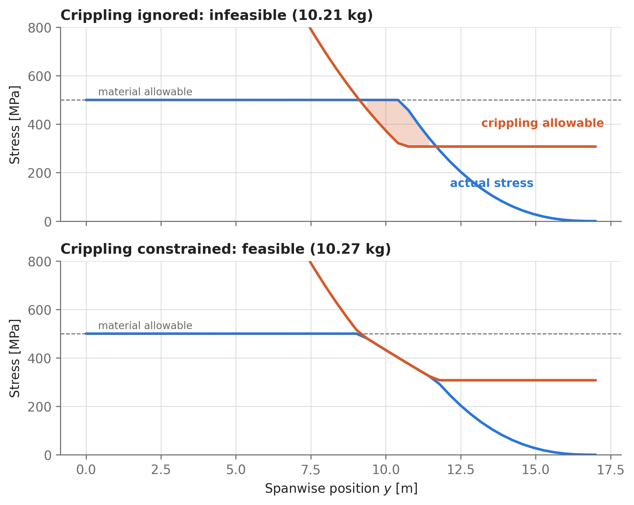
The repaired design weighs 10.27 kg — only 66 grams more (Figure 9.3). That’s the usual shape of this story: the mass cost of a forgotten failure mode is often tiny, but only the version of the design that knows about it is buildable. The general principle: any check you would run after the solve should become a constraint the moment it can fail — and because AeroSandbox models are differentiable end-to-end, promoting a check to a constraint is one subject_to() call, not a re-architecture.
9.3.2 The price of stiffness
Strength isn’t the whole story. At ultimate load, this strength-sized spar’s tip deflects 6.4 m — 38% of the half-span. Real wings usually carry some stiffness requirement too (aeroelasticity, control response, ground clearance, or simply keeping dihedral in bounds). Suppose we cap tip deflection at ultimate load to 10% of the half-span:
opti, beam, spar_mass = make_spar_problem()
opti.subject_to([
    beam.stress_axial <= crippling_allowable_stress(beam),
    beam.u[-1] <= 0.1 * half_span,  # Tip deflection limit [m]
])
sol = opti.solve(verbose=False)
mass_stiff = sol(spar_mass)
print(f"Spar mass with stiffness constraint: {mass_stiff:.2f} kg")
Spar mass with stiffness constraint: 36.29 kgThe mass explodes to 36.29 kg — 3.5\(\times\) the strength-only design. The reason is a geometry mismatch: bending stiffness scales as \(EI \propto d^3 t\), so with the diameter \(d\) frozen at 3.5 inches, the only stiffness lever left is wall thickness, and mass (\(\propto d\,t\)) grows in lockstep with it. Thickening the wall is the wrong lever; fattening the tube is the right one, since it buys stiffness cubically while costing mass only linearly. The fix is to stop dictating the diameter and let the optimizer own it — which we’ll do in Section 9.5, right after learning why an infinitely fat, infinitely thin tube isn’t free either.
9.4 Buckling: how compression members really fail
Push on the ends of a slender member and it can die three distinct deaths:
- Material failure — the stress simply exceeds what the material can take. Capacity: \(P = \sigma_\mathrm{allow} A\), independent of shape.
- Column (Euler) buckling — the whole member bows sideways as a single wave. This is a stiffness failure, not a strength failure: it depends on \(EI\) and length, not on material strength.
- Local crippling — the thin wall wrinkles locally, as in the soda can and in Section 9.3.1.
Euler’s classical formula gives the column-buckling load:
\[ P_\mathrm{cr} = \frac{\pi^2 E I}{(K L)^2} \]
where \(K\) encodes the end conditions. column_buckling_critical_load() implements this, with recommended design values of \(K\) (which are deliberately more conservative than the theoretical ones, per the AISC Steel Construction Manual):
column_buckling_critical_load()
| End conditions | Design \(K\) | Theoretical \(K\) |
|---|---|---|
| pin–pin | 1.00 | 1.00 |
| clamp–pin | 0.80 | 0.70 |
| clamp–clamp | 0.65 | 0.50 |
| clamp–free | 2.10 | 2.00 |
For the crippling mode, thin_walled_tube_crippling_buckling_critical_load() uses \(\sigma_\mathrm{crippling} = 0.3\,E t / r\) as above (pass use_recommended_design_values=False for the less conservative theoretical constant, 0.605).
The interesting engineering question is which mode governs, and the answer flips as the geometry changes. Take a concrete case: a carbon lift strut, 1.2 m long and pinned at both ends, whose cross-sectional area — and therefore mass — is fixed at 60 mm². How should we shape that fixed amount of material? Sweep the tube radius, letting the wall thin as the tube fattens:
from aerosandbox.structures.buckling import column_buckling_critical_load

L_strut = 1.2  # Strut length [m]
A = 60e-6      # Cross-sectional area of tube wall, fixed [m^2]

r = np.linspace(8e-3, 60e-3, 300)  # Tube mean radius [m]
t = A / (2 * np.pi * r)            # Wall thickness at constant area [m]

P_euler = column_buckling_critical_load(
    elastic_modulus=E,
    moment_of_inertia=np.pi * r**3 * t,  # Thin-walled tube
    length=L_strut,
    boundary_condition_type="pin-pin",
)
P_crippling = thin_walled_tube_crippling_buckling_critical_load(
    elastic_modulus=E, wall_thickness=t, radius=r,
)
P_material = stress_allowable * A * np.ones_like(r)

P_capacity = np.softmin(P_euler, P_crippling, P_material, hardness=1e9)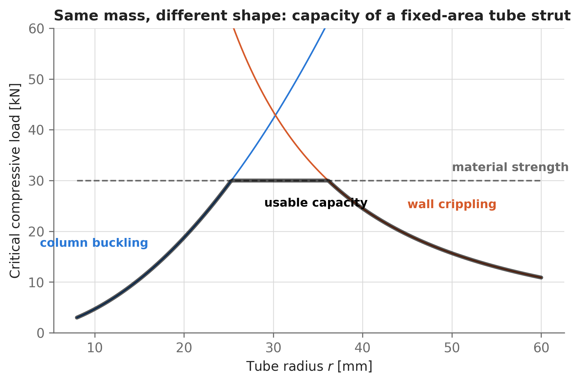
Figure 9.4 is the payoff. At small radius the strut is skinny and column buckling governs — capacity grows as \(r^2\) as the tube fattens, at zero mass cost. Past a radius of about 25 mm, material strength takes over and the capacity plateaus at 30 kN. Fatten past a radius of 36 mm — where the wall is down to 0.26 mm — and the wall becomes so thin that crippling caps the capacity, which now falls as \(1/r^2\). The design sweet spot is the plateau — and this is why aircraft compression members are fat, thin-walled tubes rather than solid rods, but only up to a point.
Note the last line of the compute cell: taking the governing mode with a raw min() would create a non-differentiable kink; np.softmin() gives a smooth version that optimizers can traverse (with hardness tuned so the blending error is negligible — see Section 3.2.2). Here we’re only plotting, but inside an Opti problem the better pattern is usually to constrain each mode separately, as we did with crippling in Section 9.3.1 — separate constraints also tell you which mode is active via the duals (Section 5.4).
9.4.1 Plate buckling
The third buckling function covers flat panels in compression — wing skins between ribs and stringers, shear-web faces, bulkhead panels. For a long plate of width \(b\) and thickness \(t\) compressed along its length, the critical stress is
\[ \sigma_\mathrm{cr} = k_c \, \frac{\pi^2 E}{12(1 - \nu^2)} \left(\frac{t}{b}\right)^2 \]
with \(k_c\) set by how the unloaded side edges are supported (\(k_c = 4.00\) simply supported, \(6.98\) clamped, \(0.425\) with one edge free — the coefficients from NACA TN 3781). For an aluminum upper-skin panel, 1.6 mm thick with 150 mm between stringers:
from aerosandbox.structures.buckling import plate_buckling_critical_load

panel_width = 0.15         # Stringer spacing [m]
panel_thickness = 1.6e-3   # Skin thickness [m]

P_cr = {
    bc: plate_buckling_critical_load(
        length=0.5,  # Rib spacing [m]; unused, as the long-plate assumption is made
        width=panel_width,
        wall_thickness=panel_thickness,
        elastic_modulus=72e9,  # Aluminum [Pa]
        poissons_ratio=0.33,
        side_boundary_condition_type=bc,
    )
    for bc in ["pin-pin", "clamp-clamp"]
}
sigma_cr = {bc: P / (panel_width * panel_thickness) for bc, P in P_cr.items()}
Simply supported, the panel buckles at just 30 MPa — a small fraction of aluminum’s strength, which is why thin skins visibly wrinkle on parked aircraft and why compression-side skins need stringers at all. Fully clamping the edges raises that to 53 MPa (1.75\(\times\)), and since real riveted or bonded joints fall between the two idealizations, the pin-pin value is the conservative design choice. Note the long-plate assumption: the returned load is independent of length and is conservative for panels shorter than a few widths.
9.5 From a physics model to a scaling law
Now let’s release the diameter, as promised in Section 9.3.2, and put everything from this chapter into one function: strength, crippling, stiffness, and gauge constraints, with the optimizer choosing a linearly tapered diameter (root and tip values — a manufacturable shape) plus the full wall-thickness distribution.
Three implementation details matter here, all instances of the robust-modeling discipline from Section 3.4. First, every variable gets a scale= matching its expected magnitude — wall thicknesses live near \(10^{-3}\) m, diameters near \(10^{-1}\) m. Second, every variable gets generous physical bounds: the upper bounds below never bind at the optimum, but without them the optimizer wanders through absurd intermediate designs (40-meter-diameter tubes) on its way there, and convergence becomes slow and fragile. Third, we pass EI_guess: when the cross-section is unknown a priori, TubeSparBendingStructure cannot infer the magnitude of the bending stiffness it should scale its internal deflection variables by, and its fallback heuristic can be off by orders of magnitude. With these three lines of hygiene, every solve in this section converges in a few dozen iterations; without them, roughly one solve in ten stalls.
def solve_spar(span, mass_total=104.0, n_ult=1.75, N=40):
    """Sizes a minimum-mass tapered tube spar. Returns (spar_mass [kg], solved beam)."""
    half_span = span / 2
    lift = n_ult * mass_total * 9.81
    d_guess = 0.01 * span  # Initial guess for diameter [m]: ~1% of span
    t_guess = 0.5e-3       # Initial guess for wall thickness [m]

    opti = asb.Opti()
    d_root = opti.variable(
        init_guess=d_guess, scale=d_guess,
        lower_bound=1e-3, upper_bound=0.02 * span,  # Generous sanity bounds
    )
    d_tip = opti.variable(
        init_guess=d_guess / 2, scale=d_guess,
        lower_bound=1e-3, upper_bound=0.02 * span,
    )
    wall_thickness = opti.variable(
        init_guess=t_guess * np.ones(N), scale=t_guess,
        lower_bound=0.2e-3, upper_bound=0.02,
    )

    beam = TubeSparBendingStructure(
        opti=opti,
        length=half_span,
        diameter_function=lambda y: d_root + (d_tip - d_root) * (y / half_span),
        wall_thickness_function=lambda y: wall_thickness,
        points_per_point_load=N,
        bending_distributed_force_function=lambda y: (lift / span)
        * (4 / np.pi) * (1 - (y / half_span) ** 2) ** 0.5,
        elastic_modulus_function=E,
        EI_guess=E * np.pi / 8 * d_guess**3 * t_guess,  # Scales internal variables
    )
    opti.subject_to([
        beam.stress_axial <= stress_allowable,
        beam.stress_axial <= crippling_allowable_stress(beam),
        beam.u[-1] <= 0.1 * half_span,  # Same stiffness requirement as before
        d_tip <= d_root,
    ])
    spar_mass = 2 * beam.volume() * rho
    opti.minimize(spar_mass)

    sol = opti.solve(verbose=False)
    return sol(spar_mass), sol(beam)


mass_free, beam_free = solve_spar(span=34.0)
print(f"Spar mass with free taper: {mass_free:.2f} kg "
      f"(root diameter {beam_free.diameter[0] * 1e3:.0f} mm, "
      f"tip {beam_free.diameter[-1] * 1e3:.0f} mm)")
Spar mass with free taper: 8.57 kg (root diameter 268 mm, tip 30 mm)At our 34-m design case, freeing the diameter drops the stiffness-constrained spar from 36.29 kg to 8.57 kg — 4.2\(\times\) lighter than the fixed-diameter version, and even 17% lighter than the strength-only design that ignored stiffness entirely. The optimizer chose a 268 mm root diameter: exactly the “fat tube, thin wall” logic of Figure 9.4, held back from going fatter still by the crippling constraint and the gauge floor.
Because each solve takes well under a second, we can afford to ask a broader question: how does optimal spar mass scale with span? This is precisely the kind of relationship a conceptual sizing study needs, and rather than assuming an exponent, we can measure it from physics:
import time

start = time.time()
spans = np.geomspace(10, 60, 9)  # Wingspans to evaluate [m]
spar_masses = np.array([solve_spar(s)[0] for s in spans])
sweep_time = time.time() - start
# Fit a power law: spar_mass = c * span^e
e_span, log_c = np.polyfit(np.log(spans), np.log(spar_masses), 1)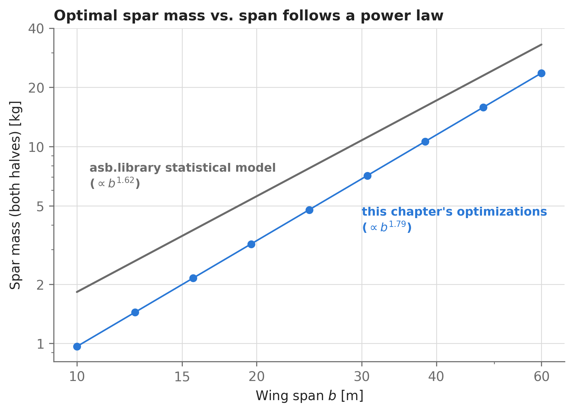
mass_wing_spar() from aerosandbox.library, which was itself generated from a sweep like this one.
All 9 optimizations ran in 7 seconds, and Figure 9.5 shows they collapse onto a nearly perfect power law with exponent 1.79: spar mass grows distinctly superlinearly with span. That exponent is the structural half of the classic induced-drag-versus-weight trade — span is aerodynamically precious (\(C_{D,i} \propto 1/b^2\)) but structurally expensive (\(m_\mathrm{spar} \propto b^{1.8}\) here), and a sizing optimizer settles where those slopes balance (Section 10.4).
The gray line is aerosandbox.library.mass_structural.mass_wing_spar(), a fitted model with a span exponent of 1.62 that ships with AeroSandbox — and it was built by exactly this workflow (the MultiBoomSparMass_v2 study in the AeroSandbox repository), just under different design rules: a fixed 0.6 mm wall with free per-station diameter, a local dihedral-angle limit instead of our tip-deflection cap, and a 570 MPa allowable. The two models agree on the structure of the relationship — power laws with similar exponents — but the library model runs 39–89% heavier across this range, precisely because its constraint set is different. That gap is a healthy reminder that there is no such thing as “the” spar mass — only the spar mass under a stated set of design rules, which is why a mass model you built, whose assumptions you can enumerate, beats one you borrowed. When your configuration matches the library model’s assumptions, use it directly (its multi-boom variants, n_booms=1..3, were generated with the legacy TubeBeam1 beam model, which also supports point loads); when it doesn’t, you now know how to build your own in an afternoon. Formal tooling for the curve-fitting step — including fits in log-space with asb.FittedModel, exactly as used for the library model — is covered in Section 17.2.
9.6 Where to go next
- Chapter 14 couples the beam model from this chapter (plus torsion) to a vortex-lattice aerodynamics solver through shared
Optivariables, computing the steady aeroelastic equilibrium of a flexible wing — MDO without an MDO framework. - Section 16.1 uses the
mass_wing_spar()scaling law from Section 9.5 inside a full solar-aircraft sizing loop, closing the mass–energy–span trade. - Section 17.2 shows how to turn sweeps like Figure 9.5 into differentiable fitted models with parameter bounds and principled residual norms.