import aerosandbox as asb
import aerosandbox.numpy as np
import aerosandbox.tools.units as u8 Atmosphere, Propulsion, and Weights
9 Atmosphere, Propulsion, and Weights
An aircraft design problem is never just aerodynamics. To close a sizing loop you also need to know what air the aircraft is flying through, what flight condition it is at, how much power the propulsion system consumes to make thrust, and how much everything weighs. This chapter covers the AeroSandbox tools for each: the asb.Atmosphere model, the asb.OperatingPoint flight-condition object, the component models in aerosandbox.library (propellers, electric powertrains, turbofans), and the statistical weight-buildup functions (Raymer, Torenbeek) together with asb.MassProperties for assembling component masses into an aircraft-level mass, CG, and inertia tensor. Everything here is differentiable and works on both plain NumPy arrays and Opti variables, so any of these models can sit inside an optimization loop — which is exactly where they end up in the design studies of Chapter 16 and Section 16.1.
9.1 The atmosphere model
Almost every quantity in flight-vehicle engineering — lift, drag, engine thrust, Reynolds number, Mach number — depends on the local air density, temperature, or pressure. AeroSandbox models these with the asb.Atmosphere class, which takes an altitude (and optionally a temperature offset) and returns the full thermodynamic state of the air.
Two methods are available:
method="isa": the 1976 International Standard Atmosphere, exactly reproduced. The ISA is piecewise-linear in temperature: constant lapse rate in the troposphere, isothermal in the lower stratosphere, and so on, with sharp corners at each layer boundary.method="differentiable"(the default): a \(C^1\)-continuous fit to the ISA. Those layer-boundary corners in the ISA are kinks — points where the derivative of temperature with respect to altitude jumps discontinuously. A gradient-based optimizer that lands near a kink sees inconsistent derivative information and can stall. The differentiable model smooths the corners while staying extremely close to the standard everywhere else, which is why it is the default.
altitude = np.linspace(0, 40e3, 500)  # [m]

atmo = asb.Atmosphere(altitude=altitude)  # differentiable model (default)
atmo_isa = asb.Atmosphere(altitude=altitude, method="isa")
Note that Atmosphere is fully vectorized: passing an array of altitudes gives arrays of properties. Figure 9.1 shows the two models overlaid — at this scale they are indistinguishable.
import _common
import matplotlib.pyplot as plt

fig, ax = plt.subplots(3, 1, figsize=(7, 7), sharex=True)

quantities = [
    ("Temperature [K]", lambda a: a.temperature()),
    ("Pressure [kPa]", lambda a: a.pressure() / 1e3),
    ("Density [kg/m$^3$]", lambda a: a.density()),
]
for a_i, (label, get) in zip(ax, quantities):
    a_i.plot(
        altitude / 1e3, get(atmo_isa),
        color=_common.TEXT_SECONDARY, linewidth=4, alpha=0.4,
    )
    a_i.plot(altitude / 1e3, get(atmo), color=_common.SERIES[0], linewidth=1.5)
    a_i.set_ylabel(label)

i_label = np.argmin(np.abs(altitude - 20e3))
T_label = atmo_isa.temperature()[i_label]
_common.label_line(ax[0], 20, T_label, "ISA (exact)", _common.TEXT_SECONDARY, dy=48)
_common.label_line(ax[0], 20, T_label, "differentiable fit", _common.SERIES[0], dy=30)
_common.annotate_event(ax[0], 11, "tropopause")
ax[-1].set_xlabel("Altitude [km]")
ax[0].set_title("The two atmosphere models are visually identical")
plt.show()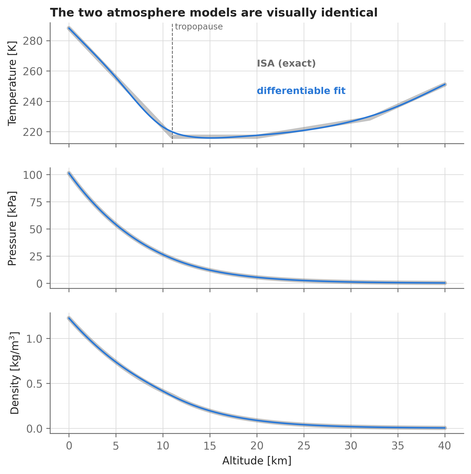
asb.Atmosphere. The exact ISA (gray) and the smoothed differentiable fit (blue) overlap at plot scale; the fit exists to remove the derivative discontinuities at ISA layer boundaries.
pressure_error = np.max(
    np.abs(atmo.pressure() - atmo_isa.pressure()) / atmo_isa.pressure()
)
Quantitatively, the differentiable model’s pressure differs from the ISA by at most 0.09% over the 0–40 km range plotted above — far smaller than the day-to-day variation of the real atmosphere. Use method="isa" when you need to reproduce standard-atmosphere table values exactly; use the default for everything else, especially anything an optimizer will touch.
9.1.1 Derived properties
Pressure and temperature are the two primary states; everything else is derived from them. The class provides speed of sound, viscosity (via Sutherland’s law), and more:
cruise_atmo = asb.Atmosphere(altitude=35e3 * u.foot)

print(f"Temperature:         {cruise_atmo.temperature():8.1f}   K")
print(f"Pressure:            {cruise_atmo.pressure():8.0f}   Pa")
print(f"Density:             {cruise_atmo.density():8.3f}   kg/m^3")
print(f"Speed of sound:      {cruise_atmo.speed_of_sound():8.1f}   m/s")
print(f"Dynamic viscosity:   {cruise_atmo.dynamic_viscosity():.3e} kg/(m*s)")
print(f"Kinematic viscosity: {cruise_atmo.kinematic_viscosity():.3e} m^2/s")
Temperature: 220.8 K
Pressure: 23848 Pa
Density: 0.376 kg/m^3
Speed of sound: 297.9 m/s
Dynamic viscosity: 1.444e-05 kg/(m*s)
Kinematic viscosity: 3.838e-05 m^2/sNote the unit-conversion idiom on the first line: aerosandbox.tools.units (imported as u) is a plain module of multiplicative conversion factors, so 35e3 * u.foot is the altitude in meters. AeroSandbox is SI-everywhere internally; u exists so you can write inputs and read outputs in whatever units your data sources use.
9.1.2 Non-standard days
The temperature_deviation argument shifts the temperature profile relative to the standard day, which matters operationally: hot air is thin air. A classic example is computing density altitude — the altitude at which the standard atmosphere would match the actual air density — at a high-elevation airport on a hot day:
# Denver (field elevation ~1,655 m) on an ISA+20°C summer afternoon:
denver_hot_day = asb.Atmosphere(
    altitude=1655,             # [m]
    temperature_deviation=20,  # [K] above standard day
)
density_altitude = denver_hot_day.density_altitude()
The airplane, whose engines and wings only care about density, behaves as if the field were at 2,359 m (7,740 ft) — roughly a kilometer higher than the airport’s true elevation. Takeoff-performance calculations that ignore this effect get people hurt.
9.2 Flight conditions: OperatingPoint
An asb.OperatingPoint bundles an Atmosphere with the aircraft’s instantaneous aerodynamic state: true airspeed velocity [m/s], angle of attack alpha [deg], sideslip beta [deg], and body rotation rates p, q, r [rad/s]. Every 3D aerodynamics analysis in AeroSandbox (Chapter 7) takes one of these as input. It also gives you the standard derived quantities of high-speed aerodynamics — dynamic pressure, Mach number, Reynolds number, and the airspeed conversions that pilots and flight-test engineers live by:
op_point = asb.OperatingPoint(
    atmosphere=asb.Atmosphere(altitude=35e3 * u.foot),
    velocity=230.0,  # true airspeed [m/s]
    alpha=2.0,       # angle of attack [deg]
)

print(f"Dynamic pressure:    {op_point.dynamic_pressure():8.0f}   Pa")
print(f"Mach number:         {op_point.mach():8.3f}")
print(f"Reynolds (4.2 m MAC): {op_point.reynolds(reference_length=4.2):.3e}")
print(f"Equivalent airspeed: {op_point.equivalent_airspeed():8.1f}   m/s")
print(f"Indicated airspeed:  {op_point.indicated_airspeed():8.1f}   m/s")
Dynamic pressure: 9953 Pa
Mach number: 0.772
Reynolds (4.2 m MAC): 2.517e+07
Equivalent airspeed: 127.5 m/s
Indicated airspeed: 137.2 m/sThe airspeed hierarchy is worth internalizing: true airspeed is the physical speed through the air; equivalent airspeed is the sea-level speed with the same dynamic pressure (what the structure feels); indicated airspeed is what a pitot-static system displays, including compressibility. At altitude, true airspeed is much higher than either.
OperatingPoint also provides convert_axes(), which transforms vectors among geometry, body, wind, and stability axes as a function of alpha and beta — the workhorse behind force bookkeeping in the aerodynamics analyses and the dynamics stack (Section 13.1).
9.2.1 A worked example: the climb crossover altitude
Jet aircraft climb at constant equivalent/indicated airspeed (a structural and control limit) until the resulting Mach number reaches the cruise Mach limit, then continue the climb at constant Mach. The altitude where the two schedules intersect is the crossover altitude. Because Atmosphere and OperatingPoint are differentiable, we can hand this directly to Opti as a one-variable root-finding problem:
rho_sea_level = asb.Atmosphere(altitude=0).density()

opti = asb.Opti()

crossover_altitude = opti.variable(init_guess=8000)  # [m]

climb_atmo = asb.Atmosphere(altitude=crossover_altitude)
true_airspeed = (280 * u.knot) / np.sqrt(climb_atmo.density() / rho_sea_level)

climb_op_point = asb.OperatingPoint(
    atmosphere=climb_atmo,
    velocity=true_airspeed,
)
opti.subject_to(climb_op_point.mach() == 0.78)

sol = opti.solve(verbose=False)
crossover_altitude = sol(crossover_altitude)

print(
    f"Crossover altitude: {crossover_altitude:,.0f} m "
    f"({crossover_altitude / u.foot:,.0f} ft)"
)
Crossover altitude: 9,199 m (30,180 ft)Figure 9.2 shows the whole climb schedule; the crossover we just solved for is where the Mach trace hits the limit.
import _common
import matplotlib.pyplot as plt

climb_altitudes = np.linspace(0, 11e3, 300)  # [m]
climb_atmo = asb.Atmosphere(altitude=climb_altitudes)
V_eas = 280 * u.knot
V_tas = V_eas / np.sqrt(climb_atmo.density() / rho_sea_level)
climb_ops = asb.OperatingPoint(atmosphere=climb_atmo, velocity=V_tas)

fig, ax = plt.subplots(2, 1, figsize=(7, 5.5), sharex=True)

ax[0].plot(
    climb_altitudes / 1e3,
    np.full_like(climb_altitudes, V_eas / u.knot),
    color=_common.TEXT_SECONDARY,
)
ax[0].plot(climb_altitudes / 1e3, V_tas / u.knot, color=_common.SERIES[0])
i_label = np.argmin(np.abs(climb_altitudes - 9e3))
_common.label_line(ax[0], 2.0, V_eas / u.knot, "equivalent airspeed",
                   _common.TEXT_SECONDARY, dy=14)
_common.label_line(ax[0], 9.0, V_tas[i_label] / u.knot, "true airspeed",
                   _common.SERIES[0], dy=-45)
ax[0].set_ylabel("Airspeed [kn]")
ax[0].set_title("Climbing at constant EAS, Mach creeps up on you")

ax[1].plot(climb_altitudes / 1e3, climb_ops.mach(), color=_common.SERIES[3])
ax[1].axhline(0.78, color=_common.TEXT_SECONDARY, linewidth=0.8, linestyle="--")
_common.label_line(ax[1], 1.0, 0.78, "Mach limit 0.78", _common.TEXT_SECONDARY, dy=0.025)
_common.annotate_event(ax[1], crossover_altitude / 1e3, "crossover")
ax[1].set_ylabel("Mach number [-]")
ax[1].set_xlabel("Altitude [km]")
plt.show()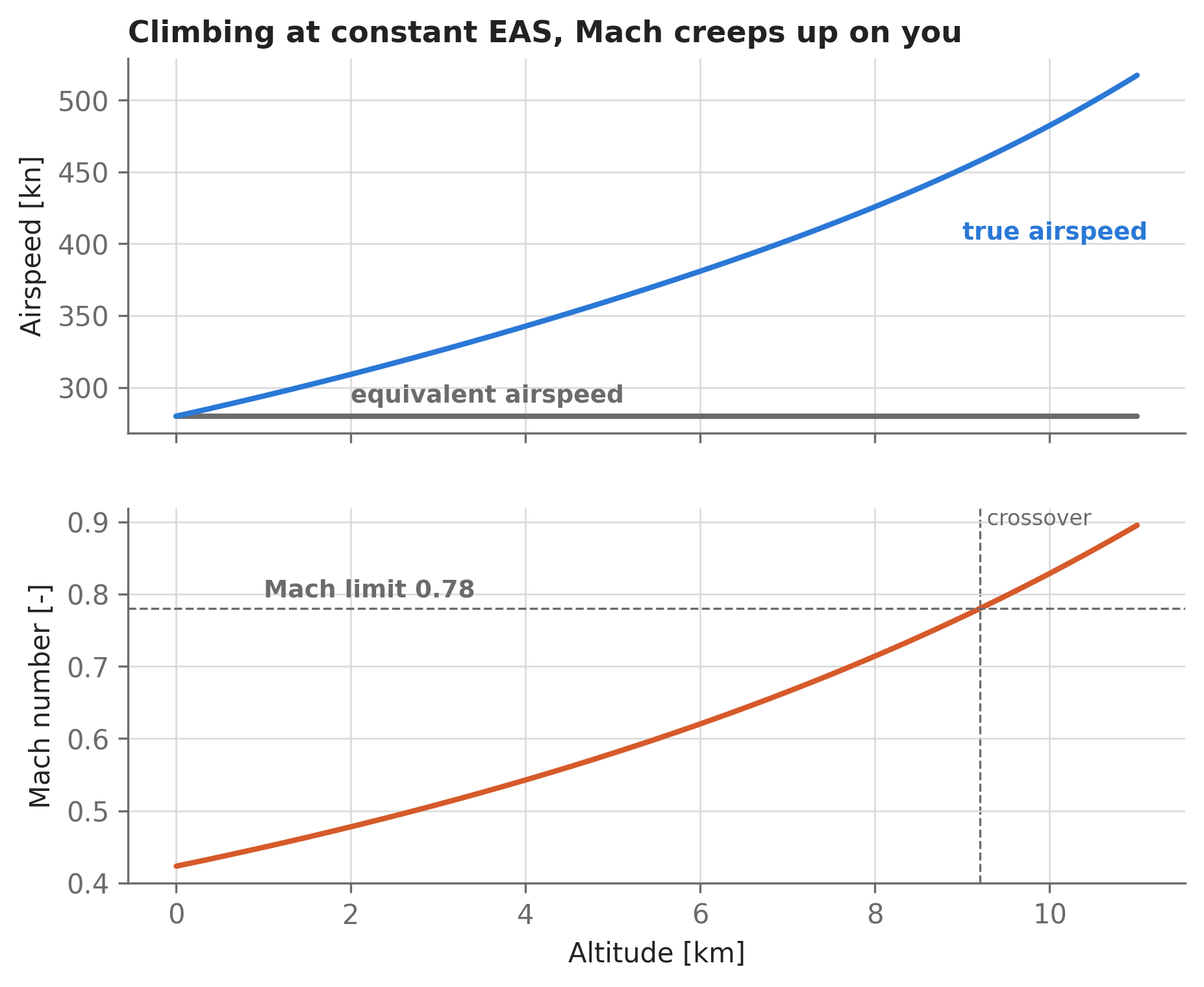
Opti constraint.
9.3 Propulsion models
aerosandbox.library is a curated collection of published, citable component models: propulsion, structural mass, solar power, gas turbines, winds aloft, costs, and more. Each is a plain differentiable function with SI inputs and outputs and a docstring citing its source. These are conceptual-design-level models — physics-based scaling laws and regressions to historical data — meant to be fast, smooth, and roughly right, so they can run thousands of times inside an optimization loop. Below is one worked example each from the propeller, electric-propulsion, and turbofan modules.
9.3.1 Propellers: actuator-disk theory
A propeller makes thrust by throwing air backwards. Momentum theory says that for a given thrust, the power required depends on disk loading — thrust per unit propeller-disk area, \(T/A\). A large, slow disk accelerates a lot of air a little (efficient); a small, highly-loaded disk accelerates a little air a lot (wasteful, because kinetic energy in the wake scales with velocity squared). propeller_shaft_power_from_thrust() implements this, plus a viscous-loss factor:
from aerosandbox.library import propulsion_propeller as lib_propeller

thrust = 400.0     # [N]
airspeed = 30.0    # [m/s]
prop_diameter = 2.0  # [m]

shaft_power = lib_propeller.propeller_shaft_power_from_thrust(
    thrust_force=thrust,
    area_propulsive=np.pi / 4 * prop_diameter**2,
    airspeed=airspeed,
    rho=asb.Atmosphere(altitude=0).density(),
    propeller_coefficient_of_performance=0.90,  # viscous (profile) losses
)
propeller_efficiency = thrust * airspeed / shaft_power

print(f"Shaft power required: {shaft_power:,.0f} W")
print(f"Propeller efficiency: {propeller_efficiency:.1%}")
Shaft power required: 14,063 W
Propeller efficiency: 85.3%Figure 9.3 sweeps this model across disk loadings: the answer to “why do human-powered airplanes and heavy-lift drones have enormous rotors” is the left side of the plot.
import _common
import matplotlib.pyplot as plt

disk_loading = np.geomspace(10, 10e3, 300)  # thrust per unit disk area [N/m²]
rho = asb.Atmosphere(altitude=0).density()

fig, ax = plt.subplots(figsize=(7, 4))
for V, color in zip([15, 30, 60], _common.SERIES):
    power_per_area = lib_propeller.propeller_shaft_power_from_thrust(
        thrust_force=disk_loading,  # thrust for a unit disk area
        area_propulsive=1.0,
        airspeed=V,
        rho=rho,
        propeller_coefficient_of_performance=0.90,
    )
    eta = disk_loading * V / power_per_area
    ax.plot(disk_loading, eta, color=color)
    _common.label_line(ax, 1.2e4, eta[-1], f"V = {V} m/s", color)

ax.set_xscale("log")
ax.set_xlim(10, 6e4)
ax.set_ylim(0, 1)
ax.set_xlabel("Disk loading $T/A$ [N/m²]")
ax.set_ylabel("Propeller efficiency [-]")
ax.set_title("Lightly-loaded disks are efficient disks")
plt.show()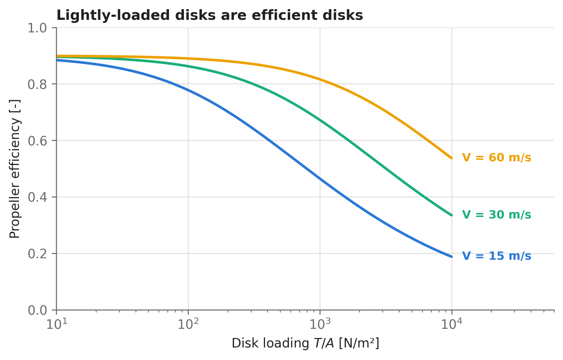
9.3.2 Electric powertrains: from battery to thrust
propulsion_electric implements Drela’s first-order motor model, which characterizes a brushless motor with just three constants: the speed constant \(K_v\), winding resistance \(R\), and no-load current \(i_0\). Given any two of {voltage, current, rpm, torque}, motor_electric_performance() solves for the rest:
from aerosandbox.library import propulsion_electric as lib_electric

motor_perf = lib_electric.motor_electric_performance(
    rpm=4000,             # operating speed
    torque=1.5,           # [N*m]
    kv=149,               # speed constant [rpm/volt]
    resistance=0.043,     # winding resistance [ohms]
    no_load_current=1.3,  # [amps]
)

for key in ["voltage", "current", "shaft power", "efficiency"]:
    print(f"{key:>12}: {motor_perf[key]:.3g}")
voltage: 27.9
current: 24.7
shaft power: 628
efficiency: 0.911For sizing studies, the higher-level electric_propeller_propulsion_analysis() chains together every element of an electric aircraft’s powertrain — propeller (the actuator-disk model above), gearbox, motor, ESC, wiring, and battery — and returns a dictionary of every intermediate quantity. Here it is for a twin-motor electric UAV in cruise:
powertrain = lib_electric.electric_propeller_propulsion_analysis(
    total_thrust=180.0,       # [N]
    n_engines=2,
    propeller_diameter=1.1,   # [m]
    op_point=asb.OperatingPoint(
        atmosphere=asb.Atmosphere(altitude=1000),
        velocity=28.0,
    ),
    motor_kv=60,              # [rpm/volt]
    motor_no_load_current=1.0,  # [A]
    motor_resistance=0.030,   # [ohms]
    wire_resistance=0.005,    # [ohms], round-trip battery-to-ESC
    battery_voltage=51.8,     # [V]
)
import pandas as pd
stages = {
"Battery output": powertrain["battery_power"],
"ESC input": powertrain["esc_electrical_power"],
"Motor electrical input": powertrain["motor_electrical_power"],
"Propeller shaft": powertrain["shaft_power"],
"Air (thrust × velocity)": powertrain["air_power"],
}
powers = list(stages.values())
pd.DataFrame(
{
"Stage": list(stages.keys()),
"Power [W]": [f"{p:,.0f}" for p in powers],
"Stage efficiency": ["—"] + [
f"{downstream / upstream:.1%}"
for upstream, downstream in zip(powers[:-1], powers[1:])
],
}
)| Stage | Power [W] | Stage efficiency | |
|---|---|---|---|
| 0 | Battery output | 6,513 | — |
| 1 | ESC input | 6,340 | 97.3% |
| 2 | Motor electrical input | 6,214 | 98.0% |
| 3 | Propeller shaft | 5,890 | 94.8% |
| 4 | Air (thrust × velocity) | 5,040 | 85.6% |
The overall battery-to-air efficiency is the product of the stage efficiencies — 77.4% here, dominated by the propeller’s 85.6%. When an electric aircraft design disappoints, look at the propeller first, not the motor: motors are already 95%-class efficient, so there is far more recoverable margin in disk loading than in copper.
9.3.3 Turbofans
For gas-turbine aircraft, propulsion_turbofan provides regressions to historical engine data plus the TASOPT engine-weight buildup from Drela. The mass model takes the thermodynamic cycle parameters you’d have at concept stage — corrected core mass flow, overall pressure ratio, bypass ratio, fan diameter — and returns the installed engine mass, including nacelle, accessories, and pylon:
from aerosandbox.library import propulsion_turbofan as lib_turbofan

# CFM56-7B26 (the 737-800 engine). Published data: dry mass 2,366 kg,
# fan diameter 1.55 m, OPR 32.7, BPR 5.1, takeoff airflow ~349 kg/s.
cfm56_dry_mass = 2366  # [kg]

installed_engine_mass = lib_turbofan.mass_turbofan(
    m_dot_core_corrected=349 / (5.1 + 1),  # core-only flow [kg/s]
    overall_pressure_ratio=32.7,
    bypass_ratio=5.1,
    diameter_fan=1.55,
)

tsfc_static = lib_turbofan.thrust_specific_fuel_consumption_turbofan(
    mass_turbofan=cfm56_dry_mass,
    bypass_ratio=5.1,
)

print(f"Installed mass estimate: {installed_engine_mass:,.0f} kg "
      f"(vs. {cfm56_dry_mass:,.0f} kg published bare-engine mass)")
print(f"Static TSFC estimate:    {tsfc_static * 1e6:.2f} mg/N/s "
      f"= {tsfc_static / (u.lbm / (u.lbf * u.hour)):.3f} lb/lbf/hr")
Installed mass estimate: 2,871 kg (vs. 2,366 kg published bare-engine mass)
Static TSFC estimate: 10.06 mg/N/s = 0.355 lb/lbf/hrBoth estimates land where they should: the installed mass exceeds the bare engine by a sensible nacelle-plus-pylon increment, and the TSFC estimate sits right at the ≈0.38 lb/lbf/hr commonly quoted for the CFM56-7B at sea-level-static conditions. (That “static” matters: TSFC grows substantially with Mach number, so cruise TSFC for this engine is closer to 0.6 lb/lbf/hr. The transport design study in Chapter 16 layers a Mach-and-altitude scaling on top of this baseline.) Figure 9.4 shows the regression’s main design story: bypass ratio buys fuel economy.
import _common
import matplotlib.pyplot as plt

bypass_ratio = np.linspace(0.5, 12, 300)

fig, ax = plt.subplots(figsize=(7, 4))
for engine_mass, label, color in [
    (2366, "CFM56-class (2,366 kg)", _common.SERIES[0]),
    (7550, "GE90-class (7,550 kg)", _common.SERIES[2]),
]:
    tsfc = lib_turbofan.thrust_specific_fuel_consumption_turbofan(
        mass_turbofan=engine_mass,
        bypass_ratio=bypass_ratio,
    ) / (u.lbm / (u.lbf * u.hour))  # convert to lb/lbf/hr for display
    ax.plot(bypass_ratio, tsfc, color=color)
    _common.label_line(ax, 6.5, tsfc[np.argmin(np.abs(bypass_ratio - 6.5))],
                       label, color, dy=0.04)

ax.set_xlabel("Bypass ratio [-]")
ax.set_ylabel("TSFC, sea-level static [lb/lbf/hr]")
ax.set_ylim(bottom=0)
ax.set_title("Bypass ratio is the big lever on fuel burn")
plt.show()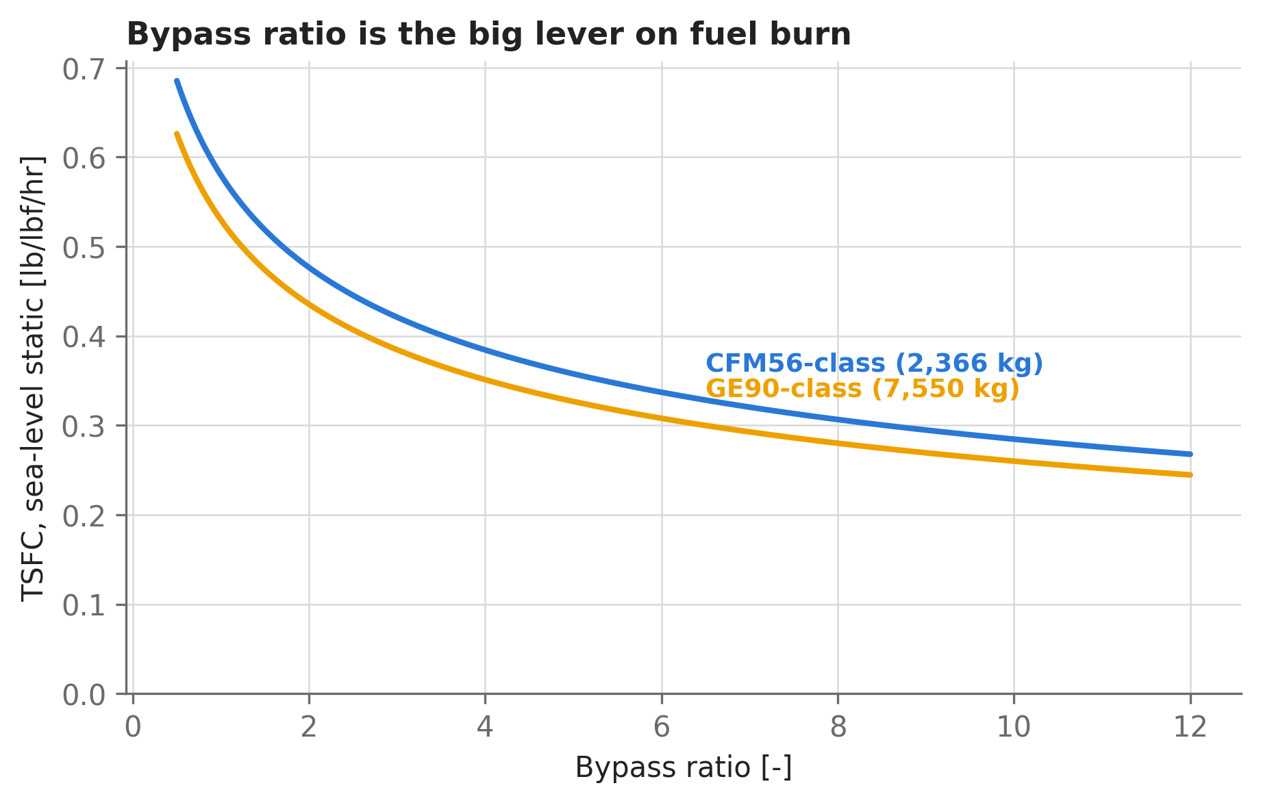
9.4 Weight buildups
At concept stage you cannot weigh hardware that doesn’t exist, so aircraft designers use statistical weight equations: regressions of component weights against the design parameters that drive them (gross weight, wing area, load factor, sweep, …), fit across fleets of existing aircraft. AeroSandbox ships the standard sets in aerosandbox.library.weights:
raymer_cargo_transport_weights— Raymer’s transport-category equations (used below),raymer_general_aviation_weights— Raymer’s GA equations, same structure, lighter aircraft,torenbeek_weights— Torenbeek’s wing and fuselage methods, which are more detailed (the wing model resolves high-lift devices, spoilers, and flutter-driven mass),nicolai_weights_light_metal_utilityandraymer_miscellaneous(seats, lavatories, passengers).
All functions take and return SI units (kilograms, meters), even though the underlying published equations are in British units — the conversions live inside. The implementations are verified term-by-term against the equations in Raymer’s text, with regression tests pinning hand-computed values. And, like everything else in this chapter, they are differentiable: if wing span is an Opti variable, wing mass responds to it, which is precisely the coupling that makes wing-sizing trades meaningful (Chapter 10).
Unlike simple scalar formulas, these functions take AeroSandbox geometry objects (asb.Wing, asb.Fuselage, asb.Airplane — see Chapter 5) and pull the spans, areas, sweeps, and control-surface layouts they need directly from them. So the first step of a weight buildup is a geometry.
9.4.1 A 737-class example
We’ll build an approximate Boeing 737-800 — a well-documented benchmark — and run the full Raymer transport buildup on it.
wing_root_airfoil = asb.Airfoil("b737b")  # actual 737 airfoils, from the UIUC database
wing_tip_airfoil = asb.Airfoil("b737d")

wing = asb.Wing(
    name="Main Wing",
    symmetric=True,
    xsecs=[
        asb.WingXSec(  # root
            xyz_le=[0, 0, 0],
            chord=6.0,
            airfoil=wing_root_airfoil,
            control_surfaces=[asb.ControlSurface(name="flap", hinge_point=0.75)],
        ),
        asb.WingXSec(  # mid-span break
            xyz_le=[4.8, 10.7, 0.65],
            chord=3.4,
            airfoil=wing_tip_airfoil,
            control_surfaces=[asb.ControlSurface(name="aileron", hinge_point=0.75)],
        ),
        asb.WingXSec(  # tip
            xyz_le=[9.6, 17.9, 1.1],
            chord=1.0,
            airfoil=wing_tip_airfoil,
        ),
    ],
).translate([13.5, 0, -1.2])

hstab = asb.Wing(
    name="Horizontal Stabilizer",
    symmetric=True,
    xsecs=[
        asb.WingXSec(
            xyz_le=[0, 0, 0],
            chord=4.0,
            airfoil=asb.Airfoil("naca0012"),
            control_surfaces=[asb.ControlSurface(name="elevator", hinge_point=0.7)],
        ),
        asb.WingXSec(xyz_le=[3.8, 7.15, 0.4], chord=1.2, airfoil=asb.Airfoil("naca0012")),
    ],
).translate([33.5, 0, 0.5])

vstab = asb.Wing(
    name="Vertical Stabilizer",
    symmetric=False,
    xsecs=[
        asb.WingXSec(
            xyz_le=[0, 0, 0],
            chord=5.2,
            airfoil=asb.Airfoil("naca0012"),
            control_surfaces=[asb.ControlSurface(name="rudder", hinge_point=0.7)],
        ),
        asb.WingXSec(xyz_le=[4.5, 0, 6.6], chord=1.5, airfoil=asb.Airfoil("naca0012")),
    ],
).translate([30.5, 0, 1.5])

fuse_length = 38.0     # [m]
fuse_radius = 3.76 / 2  # [m]

def fuselage_radius(x):
    if x < 6:  # nose taper
        return fuse_radius * (1 - ((x - 6) / 6) ** 2) ** 0.5
    elif x > fuse_length - 12:  # tail taper
        return fuse_radius * (1 - 0.85 * ((x - (fuse_length - 12)) / 12) ** 1.5)
    else:  # constant cabin section
        return fuse_radius

fuselage = asb.Fuselage(
    name="Fuselage",
    xsecs=[
        asb.FuselageXSec(xyz_c=[x, 0, 0], radius=fuselage_radius(x))
        for x in np.sinspace(0, fuse_length, 30)
    ],
)

airplane = asb.Airplane(
    name="737-800-class",
    wings=[wing, hstab, vstab],
    fuselages=[fuselage],
)

print(f"Wing area:    {wing.area():.1f} m^2")
print(f"Aspect ratio: {wing.aspect_ratio():.2f}")
print(f"1/4-chord sweep: {wing.mean_sweep_angle():.1f} deg")
Wing area: 132.5 m^2
Aspect ratio: 9.71
1/4-chord sweep: 25.0 degairplane.draw_three_view()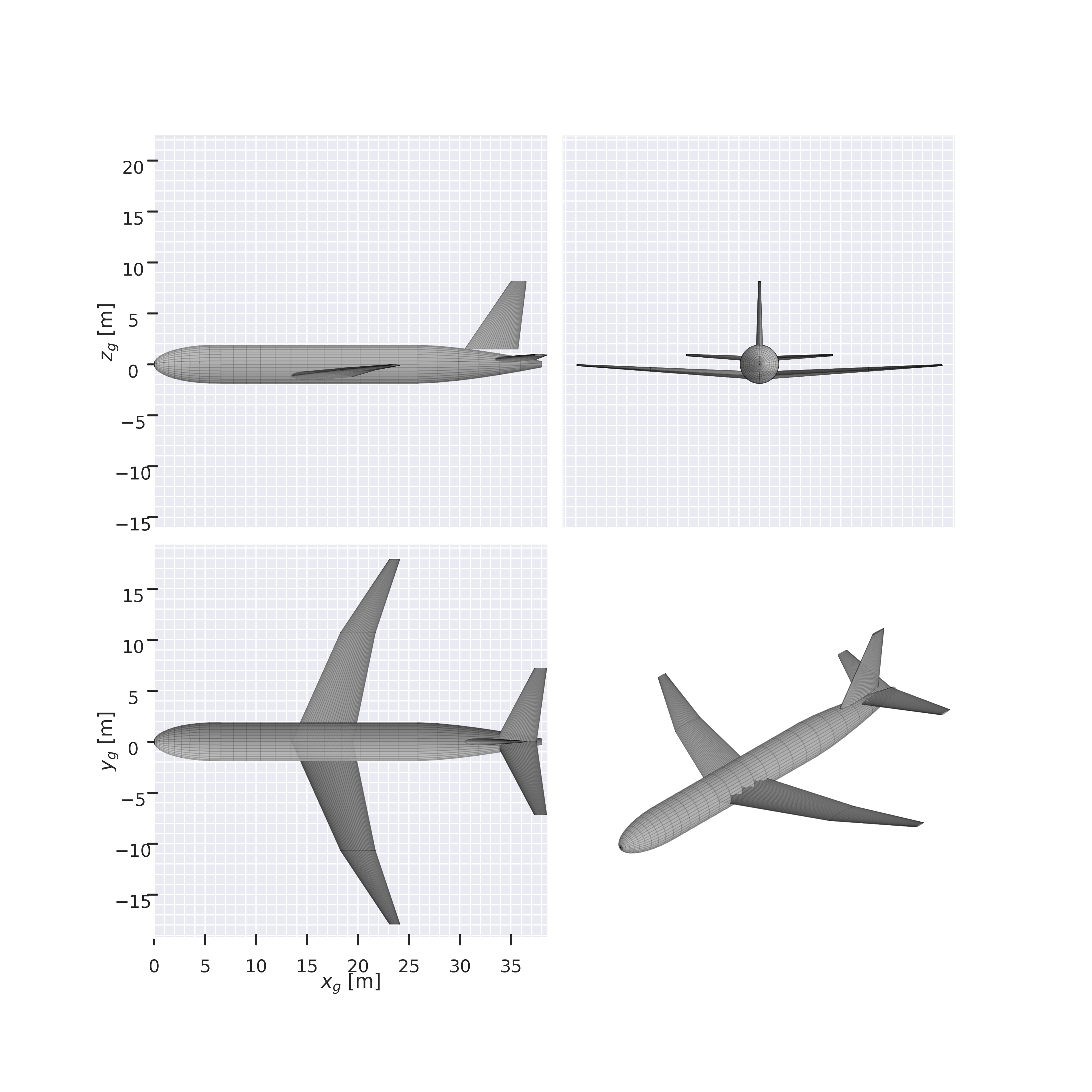
array([[<Axes3D: zlabel='$z_g$ [m]'>, <Axes3D: >],
       [<Axes3D: xlabel='$x_g$ [m]', ylabel='$y_g$ [m]'>, <Axes3D: >]],
dtype=object)<module '_common' from '/tmp/claude-1000/-home-psharpe-gh-AeroSandbox/1ccf6b40-3256-4f8d-9484-ebe00c7e55db/scratchpad/book-staging/_common.py'>Next, the top-level design assumptions. These are the quantities Raymer’s equations key on but that don’t live in the geometry:
design_mass_TOGW = 79000        # [kg] max takeoff mass, 737-800 class
ultimate_load_factor = 1.5 * 2.5  # 2.5g limit load × 1.5 safety factor
n_pax = 189                     # single-class seating
mass_per_engine = 2366          # [kg] CFM56-7B26 dry mass
Now the buildup itself, component by component. Group one — structure:
from aerosandbox.library.weights import raymer_cargo_transport_weights as raymer_ct
from aerosandbox.library.weights import raymer_miscellaneous as raymer_misc

structure = {
    "Wing": raymer_ct.mass_wing(
        wing=wing,
        design_mass_TOGW=design_mass_TOGW,
        ultimate_load_factor=ultimate_load_factor,
    ),
    "Horizontal stabilizer": raymer_ct.mass_hstab(
        hstab=hstab,
        design_mass_TOGW=design_mass_TOGW,
        ultimate_load_factor=ultimate_load_factor,
        wing_to_hstab_distance=(
            hstab.aerodynamic_center()[0] - wing.aerodynamic_center()[0]
        ),
        fuselage_width_at_hstab_intersection=0.7 * 2 * fuse_radius,
    ),
    "Vertical stabilizer": raymer_ct.mass_vstab(
        vstab=vstab,
        design_mass_TOGW=design_mass_TOGW,
        ultimate_load_factor=ultimate_load_factor,
        wing_to_vstab_distance=(
            vstab.aerodynamic_center()[0] - wing.aerodynamic_center()[0]
        ),
    ),
    "Fuselage": raymer_ct.mass_fuselage(
        fuselage=fuselage,
        design_mass_TOGW=design_mass_TOGW,
        ultimate_load_factor=ultimate_load_factor,
        L_over_D=17,
        main_wing=wing,
    ),
    "Main landing gear": raymer_ct.mass_main_landing_gear(
        main_gear_length=1.8,
        landing_speed=71,
        design_mass_TOGW=design_mass_TOGW,
        n_gear=2,
        n_wheels=4,
        n_shock_struts=2,
    ),
    "Nose landing gear": raymer_ct.mass_nose_landing_gear(
        nose_gear_length=1.3,
        design_mass_TOGW=design_mass_TOGW,
        n_gear=1,
        n_wheels=2,
    ),
}
Group two — propulsion. The engines themselves come from published data (or the TASOPT mass model of the previous section); Raymer’s equations cover the installation: nacelles, engine controls, starters, and the fuel system.
propulsion = {
    "Engines (dry, ×2)": 2 * mass_per_engine,
    "Nacelles": raymer_ct.mass_nacelles(
        nacelle_length=4.3,
        nacelle_width=2.1,
        nacelle_height=2.1,
        ultimate_load_factor=ultimate_load_factor,
        mass_per_engine=mass_per_engine,
        n_engines=2,
        is_pylon_mounted=True,
        engines_have_thrust_reversers=True,
    ),
    "Engine controls": raymer_ct.mass_engine_controls(
        n_engines=2,
        cockpit_to_engine_length=18,
    ),
    "Engine starters": raymer_ct.mass_starter(
        n_engines=2,
        mass_per_engine=mass_per_engine,
    ),
    "Fuel system": raymer_ct.mass_fuel_system(
        fuel_volume=26e3 * u.liter,
        n_tanks=3,
    ),
}
Group three — systems and equipment:
systems = {
    "Flight controls": raymer_ct.mass_flight_controls(
        airplane=airplane,
        aircraft_Iyy=design_mass_TOGW * (0.25 * fuse_length) ** 2,  # gyradius guess
    ),
    "APU": raymer_ct.mass_APU(mass_APU_uninstalled=145),
    "Instruments": raymer_ct.mass_instruments(
        fuselage=fuselage, main_wing=wing, n_engines=2, n_crew=2,
    ),
    "Hydraulics": raymer_ct.mass_hydraulics(
        airplane=airplane, fuselage=fuselage, main_wing=wing,
    ),
    "Electrical": raymer_ct.mass_electrical(
        system_electrical_power_rating=50e3,  # [W]
        electrical_routing_distance=30,       # [m]
        n_engines=2,
    ),
    "Avionics": raymer_ct.mass_avionics(mass_uninstalled_avionics=1000 * u.lbm),
    "Air conditioning": raymer_ct.mass_air_conditioning(
        n_crew=6,
        n_pax=n_pax,
        volume_pressurized=np.pi * fuse_radius**2 * 30,  # [m^3]
        mass_uninstalled_avionics=1000 * u.lbm,
    ),
    "Anti-ice": raymer_ct.mass_anti_ice(design_mass_TOGW=design_mass_TOGW),
    "Handling gear": raymer_ct.mass_handling_gear(design_mass_TOGW=design_mass_TOGW),
}

furnishings = {
    "Furnishings": raymer_ct.mass_furnishings(
        n_crew=6,
        mass_cargo=20e3,  # [kg] max payload
        fuselage=fuselage,
    ),
    "Seats": (
        n_pax * raymer_misc.mass_seat("passenger")
        + 2 * raymer_misc.mass_seat("flight_deck")
    ),
    "Lavatories": raymer_misc.mass_lavatories(
        n_pax=n_pax, aircraft_type="short-haul",
    ),
}

masses = {**structure, **propulsion, **systems, **furnishings}
empty_mass = sum(masses.values())
Table 9.2 collects the result, and Figure 9.6 shows it graphically.
import pandas as pd

groups = {
    **{k: "Structure" for k in structure},
    **{k: "Propulsion" for k in propulsion},
    **{k: "Systems" for k in systems},
    **{k: "Furnishings" for k in furnishings},
}
weights_table = pd.DataFrame(
    {
        "Group": [groups[k] for k in masses],
        "Component": list(masses.keys()),
        "Mass [kg]": [f"{m:,.0f}" for m in masses.values()],
        "Fraction of empty mass": [f"{m / empty_mass:.1%}" for m in masses.values()],
    }
)
weights_table| Group | Component | Mass [kg] | Fraction of empty mass | |
|---|---|---|---|---|
| 0 | Structure | Wing | 6,839 | 21.2% |
| 1 | Structure | Horizontal stabilizer | 717 | 2.2% |
| 2 | Structure | Vertical stabilizer | 549 | 1.7% |
| 3 | Structure | Fuselage | 7,084 | 21.9% |
| 4 | Structure | Main landing gear | 2,832 | 8.8% |
| 5 | Structure | Nose landing gear | 374 | 1.2% |
| 6 | Propulsion | Engines (dry, ×2) | 4,732 | 14.6% |
| 7 | Propulsion | Nacelles | 1,223 | 3.8% |
| 8 | Propulsion | Engine controls | 47 | 0.1% |
| 9 | Propulsion | Engine starters | 79 | 0.2% |
| 10 | Propulsion | Fuel system | 399 | 1.2% |
| 11 | Systems | Flight controls | 721 | 2.2% |
| 12 | Systems | APU | 319 | 1.0% |
| 13 | Systems | Instruments | 93 | 0.3% |
| 14 | Systems | Hydraulics | 83 | 0.3% |
| 15 | Systems | Electrical | 370 | 1.1% |
| 16 | Systems | Avionics | 698 | 2.2% |
| 17 | Systems | Air conditioning | 935 | 2.9% |
| 18 | Systems | Anti-ice | 158 | 0.5% |
| 19 | Systems | Handling gear | 24 | 0.1% |
| 20 | Furnishings | Furnishings | 1,081 | 3.3% |
| 21 | Furnishings | Seats | 2,798 | 8.7% |
| 22 | Furnishings | Lavatories | 150 | 0.5% |
import _common
import matplotlib.pyplot as plt

group_colors = {
    "Structure": _common.SERIES[0],
    "Propulsion": _common.SERIES[2],
    "Systems": _common.SERIES[1],
    "Furnishings": _common.SERIES[4],
}
sorted_items = sorted(masses.items(), key=lambda kv: kv[1])

fig, ax = plt.subplots(figsize=(7, 6))
ax.barh(
    [k for k, v in sorted_items],
    [v for k, v in sorted_items],
    color=[group_colors[groups[k]] for k, v in sorted_items],
)
for i, (k, v) in enumerate(sorted_items):
    ax.text(v * 1.1, i, f"{v:,.0f}", va="center", fontsize=8,
            color=_common.TEXT_SECONDARY)
ax.set_xscale("log")
ax.set_xlim(right=3e4)
ax.set_xlabel("Component mass [kg], log scale")
for group, color in group_colors.items():
    ax.scatter([], [], color=color, label=group)
ax.legend(loc="lower right", fontsize=9)
ax.set_title("Wing, fuselage, and engines dominate the empty mass")
plt.show()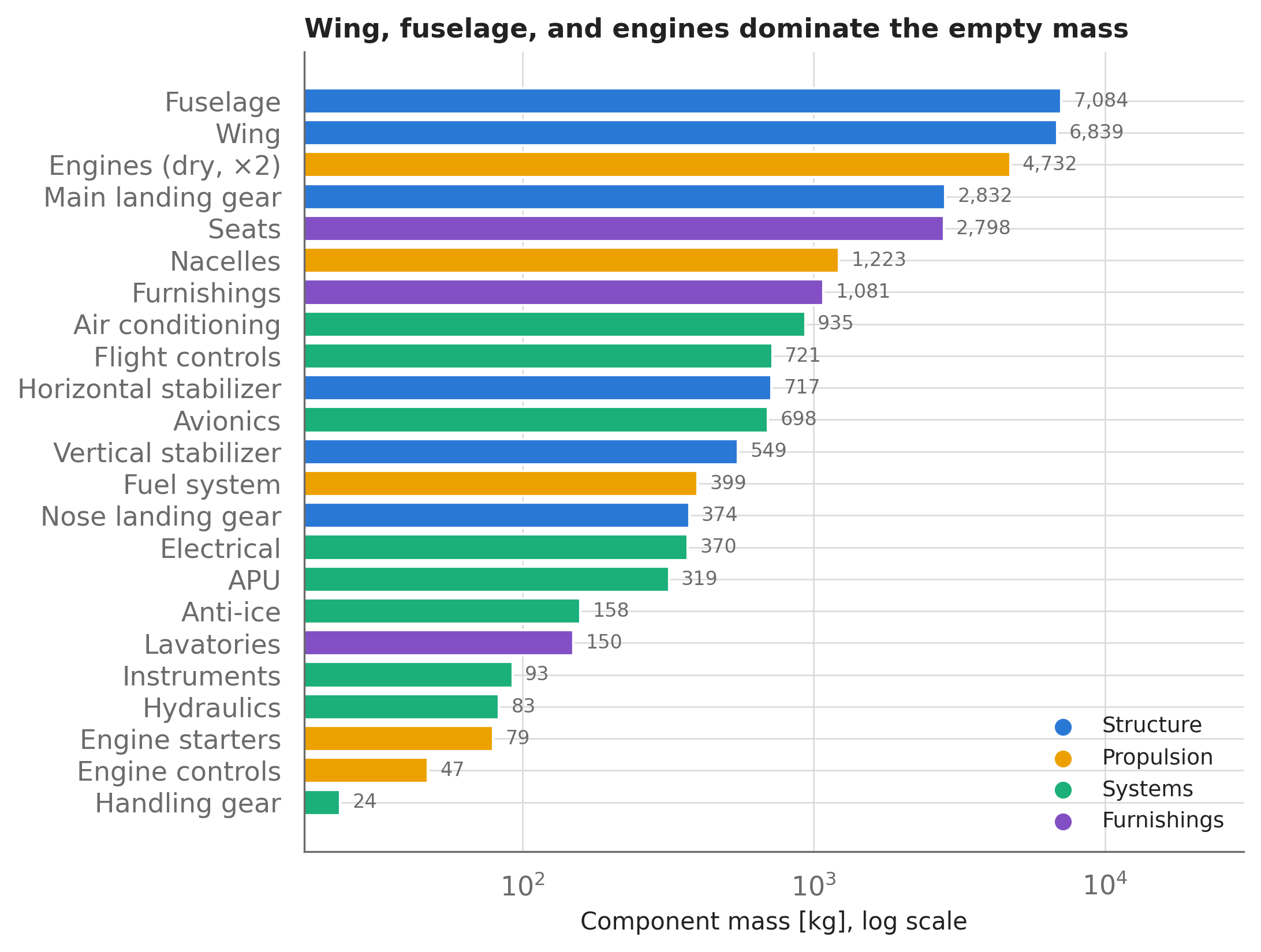
How good is the total? The published operating empty weight of a 737-800 is about 41,400 kg. Our buildup gives:
oew_published = 41400  # [kg] 737-800 operating empty weight, published

print(f"Empty-mass buildup:  {empty_mass:,.0f} kg")
print(f"Published 737-800 OEW: {oew_published:,.0f} kg")
print(f"Ratio: {empty_mass / oew_published:.1%}")
Empty-mass buildup: 32,304 kg
Published 737-800 OEW: 41,400 kg
Ratio: 78.0%Landing about 22% low is typical, and understanding why is part of learning to use weight equations. First, operating empty weight includes several tonnes of items this buildup deliberately excludes: crew and their bags, galleys and catering equipment, potable water, emergency equipment, unusable fuel, paint. Second, the individual regressions carry real scatter — cross-checking the wing against Torenbeek’s more detailed method illustrates the model-form uncertainty:
from aerosandbox.library.weights import torenbeek_weights as torenbeek

wing_mass_torenbeek = torenbeek.mass_wing(
    wing=wing,
    design_mass_TOGW=design_mass_TOGW,
    ultimate_load_factor=ultimate_load_factor,
    suspended_mass=design_mass_TOGW - structure["Wing"],
    never_exceed_airspeed=200,       # [m/s], EAS
    max_airspeed_for_flaps=115,      # [m/s]
    main_gear_mounted_to_wing=True,
)

print(f"Wing mass, Raymer:    {structure['Wing']:,.0f} kg")
print(f"Wing mass, Torenbeek: {wing_mass_torenbeek:,.0f} kg")
Wing mass, Raymer: 6,839 kg
Wing mass, Torenbeek: 8,315 kgTwo respected methods disagree by +22% on the single heaviest structural component. The practical lessons: (1) always calibrate a weight buildup against a known aircraft of the same class before trusting it on your design, and (2) treat component weights as uncertain inputs to be swept, not truths. When you do have a systematic bias you trust — say, a composite airframe versus the mostly-metal historical fleet these regressions were fit on — apply it explicitly: each structural function accepts use_advanced_composites=True, which applies the correction factors from raymer_fudge_factors (about a 10–15% credit, depending on the component).
For lighter aircraft, raymer_general_aviation_weights provides the same buildup with equations fit to the GA fleet — same call style, same SI conventions.
9.5 Assembling mass properties
A weight buildup gives component masses; an aircraft model also needs to know where that mass is — the center of gravity drives stability and control, and the inertia tensor drives dynamics. asb.MassProperties handles the bookkeeping. Each instance stores a mass, a CG location, and an inertia tensor about that CG, and instances add: summing two MassProperties objects returns the combined mass, the mass-weighted CG, and the combined inertia tensor with all parallel-axis terms applied automatically.
So the whole aircraft-level calculation is: attach a location to each component from the table above, and sum.
# Wing-anchored reference quantities, for CG bookkeeping in %MAC:
mac = wing.mean_aerodynamic_chord()                    # [m]
x_lemac = wing.aerodynamic_center()[0] - 0.25 * mac    # leading edge of MAC [m]
x_cabin_mid = 0.45 * fuse_length

x_cg_map = {  # [m] aft of the nose; typical component CG stations
    "Wing": x_lemac + 0.40 * mac,
    "Horizontal stabilizer": hstab.aerodynamic_center()[0] + 0.15 * hstab.mean_aerodynamic_chord(),
    "Vertical stabilizer": vstab.aerodynamic_center()[0] + 0.15 * vstab.mean_aerodynamic_chord(),
    "Fuselage": 0.45 * fuse_length,
    "Main landing gear": x_lemac + 0.60 * mac,
    "Nose landing gear": 4.5,
    "Engines (dry, ×2)": 12.5,
    "Nacelles": 12.5,
    "Engine controls": 10.0,
    "Engine starters": 12.5,
    "Fuel system": x_lemac + 0.45 * mac,
    "Flight controls": 25.0,
    "APU": 36.5,
    "Instruments": 3.5,
    "Hydraulics": 20.0,
    "Electrical": 10.0,
    "Avionics": 3.5,
    "Air conditioning": x_cabin_mid,
    "Anti-ice": x_lemac + 0.40 * mac,
    "Handling gear": x_cabin_mid,
    "Furnishings": x_cabin_mid,
    "Seats": x_cabin_mid,
    "Lavatories": x_cabin_mid,
}

mass_props = {
    name: asb.MassProperties(mass=m, x_cg=x_cg_map[name])
    for name, m in masses.items()
}
Modeling each component as a point mass captures the CG exactly and much of the inertia (the parallel-axis terms), but misses each component’s inertia about its own CG. Where that matters — long, distributed components like the fuselage — use mass_properties_from_radius_of_gyration():
mass_props["Fuselage"] = asb.mass_properties_from_radius_of_gyration(
    mass=masses["Fuselage"],
    x_cg=x_cg_map["Fuselage"],
    radius_of_gyration_y=fuse_length / 12**0.5,  # slender-rod approximation
    radius_of_gyration_z=fuse_length / 12**0.5,
)

empty_mass_props = sum(mass_props.values())
empty_mass_props
MassProperties instance:
Mass : 32304.023
Center of Gravity : ( 17.266343, 0, 0)
Inertia Tensor :
(about CG) [ 0, 0, 0]
[ 0, 1814668.1, 0]
[ 0, 0, 1814668.1]empty_cg_percent_mac = (empty_mass_props.x_cg - x_lemac) / macThe empty CG lands at 12% MAC — forward of the wing’s aerodynamic center at 25% MAC, as it should be for an empty transport (payload and fuel then shift it within the loadable envelope). Figure 9.7 shows where each component sits and how the pieces balance.
import _common
import matplotlib.pyplot as plt

fig, ax = plt.subplots(figsize=(7, 4.5))
ax.axvspan(x_lemac, x_lemac + mac, color=_common.GRID, alpha=0.5, zorder=0)
ax.text(x_lemac + mac / 2, 12, "MAC", color=_common.TEXT_SECONDARY,
        ha="center", fontsize=8)

for name, m in masses.items():
    ax.scatter(x_cg_map[name], m, color=group_colors[groups[name]], s=25, zorder=3)
ax.axvline(empty_mass_props.x_cg, color=_common.SERIES[3], linewidth=1.5)
_common.label_line(ax, empty_mass_props.x_cg, 2.2e4, " empty CG", _common.SERIES[3])

for name, ha, dx, dy in [("Wing", "left", 0.7, 1.0), ("Fuselage", "right", -0.7, 1.0),
                         ("Engines (dry, ×2)", "right", -0.7, 1.0),
                         ("APU", "right", -0.7, 1.0),
                         ("Nose landing gear", "center", 0, 0.72)]:
    ax.annotate(name, (x_cg_map[name] + dx, masses[name] * dy),
                fontsize=8, ha=ha, va="center", color=_common.TEXT_SECONDARY)

ax.set_yscale("log")
ax.set_ylim(8, 3e4)
ax.set_xlabel("Longitudinal station, aft of nose [m]")
ax.set_ylabel("Component mass [kg], log scale")
ax.set_title("Where the mass lives")
plt.show()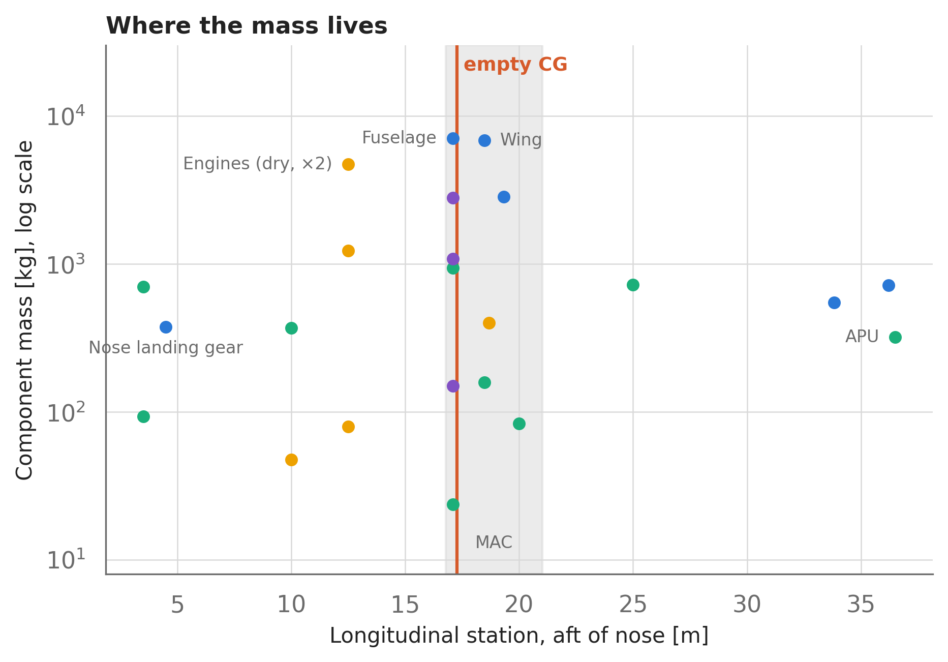
Because MassProperties supports arithmetic (+, and * by a scalar), loading studies are just more algebra: add a MassProperties for fuel at the tank CG and one for payload at the cabin CG to get gross-weight CG and inertia, and sweep the fuel state to trace the CG envelope. The dynamics stack (Section 13.1) consumes these same objects directly, and helpers exist for common shapes (mass_properties_of_ellipsoid(), mass_properties_of_rectangular_prism(), …) when you’d rather derive inertias than assume gyradii.
9.6 Where to go next
- Chapter 16 puts everything in this chapter to work at once: a full transport-aircraft sizing loop where a Raymer-style weight buildup, engine scaling, and the atmosphere model close a takeoff-gross-weight iteration inside one
Optiproblem. - Chapter 11 is the compact version of the same idea — aero, weights, and range closure in a problem small enough to read in one sitting.
- Section 13.1 shows where
OperatingPointandMassPropertiesgo next: full flight-dynamics simulation and trajectory optimization.