import aerosandbox as asb
import aerosandbox.numpy as np5 Defining Aircraft Geometry
Everything in AeroSandbox that analyzes, draws, or optimizes an aircraft starts from one data structure: the asb.Airplane object. An Airplane is a nested tree — wings, fuselages, and propulsors, each built from 2D cross-sections, which are in turn built from airfoils and a handful of scalar dimensions. Define the geometry once, and the same object feeds every analysis in the library: the drag buildup, the vortex-lattice solver, the stability-derivative calculator, and the AVL/XFLR5/OpenVSP/CAD exporters. Crucially, every scalar in the tree — a chord, a twist angle, a cross-section location — can be either a plain number or an optimization variable, which is what makes AeroSandbox geometry optimization-native rather than merely scriptable.
In this chapter, we build a complete airplane — a Cessna 152-class two-seat trainer — from the ground up: airfoils, wing cross-sections, control surfaces, a fuselage, a propeller disk, and the assembled Airplane with its three-view drawing. Along the way we extract the derived quantities that every design calculation needs (reference area, aspect ratio, mean aerodynamic chord, wetted areas), attach mass properties with the asb.MassProperties algebra, and end with a five-line demonstration of geometry-in-the-optimizer.
5.1 The geometry tree and its conventions
An AeroSandbox airplane is a tree of components, and each lofted component is a list of cross-sections (“xsecs”):
Airplanewings: list[Wing]— eachWingis a list ofWingXSeccross-sections, lofted root-to-tip. EachWingXSeccarries anAirfoil.fuselages: list[Fuselage]— eachFuselageis a list ofFuselageXSeccross-sections, lofted nose-to-tail.propulsors: list[Propulsor]— disks or cylinders representing propellers, rotors, or engines.
Users familiar with MIT’s AVL will recognize this structure — it is nearly identical to AVL’s surface/section hierarchy, which has been the lingua franca of conceptual-design aerodynamics for decades.
ImportantConventions: axes, units, angles
Geometry is defined in geometry axes: \(x\) points aft (toward the tail), \(y\) points out the right wing, and \(z\) points up. This is body axes rotated 180° about \(y\). The origin is wherever you like; a common choice (used in this chapter) is the leading edge of the wing root.
All lengths are in meters and all angles are in degrees, everywhere in AeroSandbox. If your source data is in feet, knots, or pounds, convert at the boundary with aerosandbox.tools.units — never store non-SI values inside the geometry.
Standard imports for everything that follows:
5.2 Airfoils
The leaf node of the geometry tree is the asb.Airfoil: a named 2D shape, stored as an ordered array of \((x/c,\ y/c)\) coordinates that wrap from the upper-surface trailing edge, around the nose, and back to the lower-surface trailing edge. You rarely need to supply coordinates yourself — the constructor can generate or look them up by name:
af = asb.Airfoil("naca2412")  # 4-digit NACA sections are generated analytically
af
Airfoil naca2412 (399 points)Three ways to make an airfoil, in order of decreasing convenience:
- By name. 4- and 5-digit NACA sections (
"naca2412","naca23012") are generated from the defining equations; anything else ("dae11","sd7037","e216", …) is looked up in the bundled copy of the UIUC airfoil database — the string must match the database’s.datfilename. - From a file:
asb.Airfoil(name="MyFoil", coordinates="path/to/foil.dat")reads a Selig-format.datfile. - From an array: pass an
(N, 2)NumPy array of coordinates directly.
A quick look at the section, with its mean camber line:
af.draw(draw_mcl=True)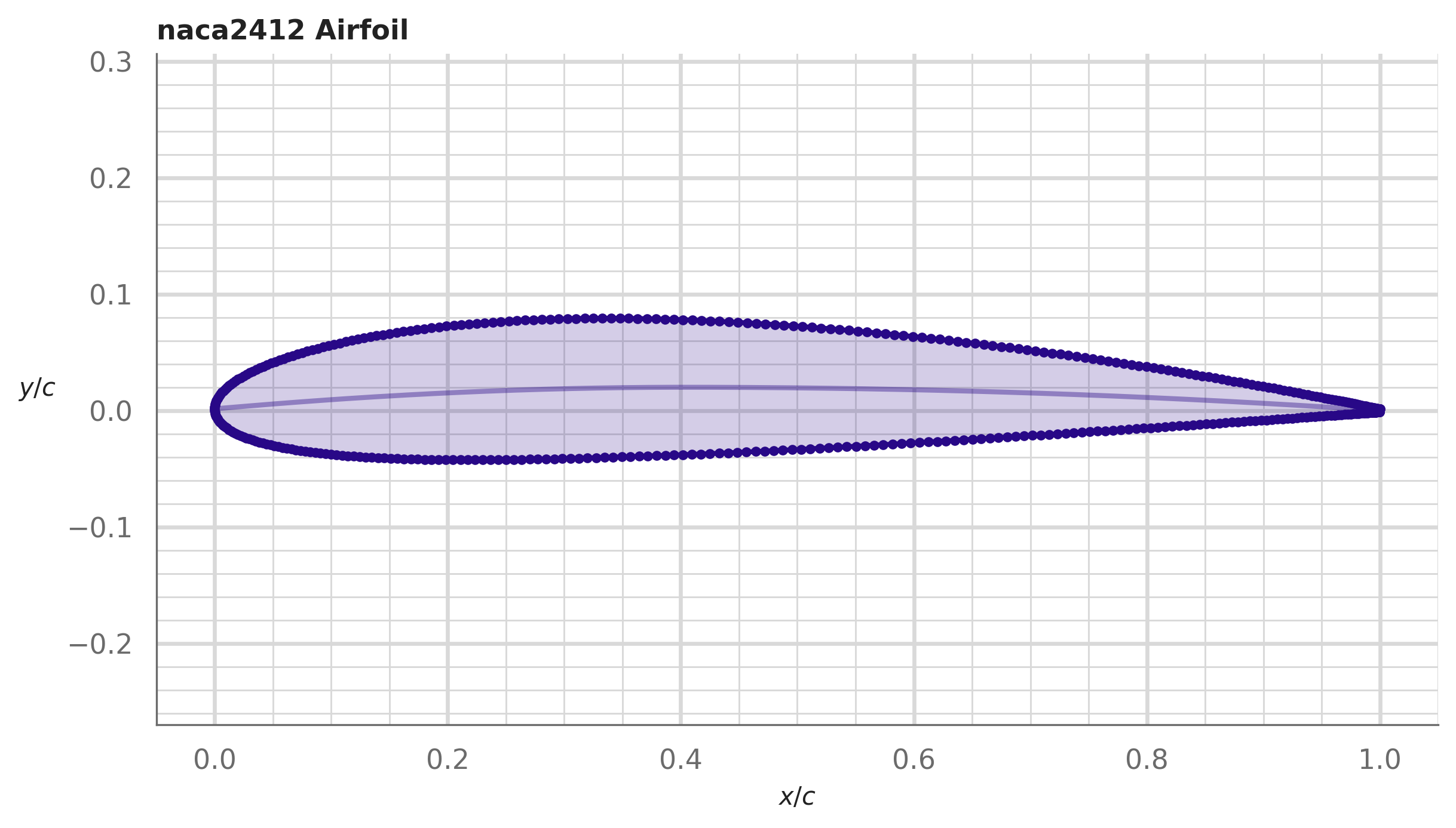
Airfoil.draw(). The faint interior line is the mean camber line.
Because an Airfoil is fundamentally a polygon, it knows its own geometric properties — no lookup tables required:
print(f"Max thickness:      {af.max_thickness():.4f} (t/c, at max)")
print(f"Max camber:         {af.max_camber():.4f}")
print(f"Cross-section area: {af.area():.4f} (normalized by chord^2)")
print(f"Perimeter:          {af.perimeter():.4f} (normalized by chord)")
print(f"LE radius:          {af.LE_radius():.4f} (normalized by chord)")
print(f"TE angle:           {af.TE_angle():.2f} deg")
Max thickness: 0.1201 (t/c, at max)
Max camber: 0.0200
Cross-section area: 0.0823 (normalized by chord^2)
Perimeter: 2.0439 (normalized by chord)
LE radius: 0.0157 (normalized by chord)
TE angle: 15.94 degThese feed directly into design math: area() scales fuel-volume and spar-depth estimates, perimeter() sets wetted area (a wing’s wetted area is the sum over sections of chord × perimeter), and local_thickness(x_over_c) is handy for lofting bodies of revolution — we’ll use exactly that trick for a fuselage-like shape later. Utility methods like repanel(), scale(), rotate(), and blend_with_another_airfoil() cover the day-to-day manipulations; aerodynamic performance (lift, drag, moment polars via NeuralFoil) is the subject of Chapter 6.
5.2.1 The Kulfan (CST) parameterization
Raw coordinate arrays are a poor design space: hundreds of coordinates means hundreds of optimization variables, and wiggling any one of them independently produces noisy, non-smooth shapes. What an optimizer wants is a low-dimensional, smooth parameterization where every parameter combination yields a sensible airfoil. AeroSandbox’s answer is asb.KulfanAirfoil, which implements the Kulfan Class/Shape Transformation (CST) parameterization: each surface is a smooth analytic “class function” (round nose, sharp tail) multiplied by a Bernstein-polynomial “shape function” controlled by 8 weights per surface, plus one leading-edge weight and a trailing-edge thickness — 18 numbers total for a typical airfoil.
Any coordinate airfoil can be fit:
dae11 = asb.Airfoil("dae11")            # a cambered high-lift section, from coordinates
dae11_k = dae11.to_kulfan_airfoil()     # least-squares CST fit
dae11_k.kulfan_parameters["upper_weights"]
array([0.17036014, 0.15272658, 0.51688551, 0.09212467, 0.66904449,
0.14345864, 0.28990386, 0.16207357])(You can also construct one directly by name — asb.KulfanAirfoil("dae11") — or from explicit weight vectors.) The fit is essentially exact for engineering purposes, and the weights are interpretable knobs: scaling the upper-surface weights inflates the upper surface; the leading-edge weight blunts or sharpens the nose.
import _common
import matplotlib.pyplot as plt

fig, axs = plt.subplots(2, 1, figsize=(7, 5.5))

### Top panel: fit quality on the DAE-11
ax = axs[0]
ax.plot(
    dae11.coordinates[:, 0], dae11.coordinates[:, 1],
    ".", color=_common.TEXT_SECONDARY, markersize=5,
)
kc = dae11_k.coordinates
ax.plot(kc[:, 0], kc[:, 1], color=_common.SERIES[0], linewidth=1.5)

# Fit error: evaluate the CST fit at the original coordinates' x-locations
n_up = dae11.LE_index() + 1
y_err = np.concatenate([
    dae11_k.upper_coordinates(dae11.coordinates[:n_up, 0])[:, 1]
    - dae11.coordinates[:n_up, 1],
    dae11_k.lower_coordinates(dae11.coordinates[n_up:, 0])[:, 1]
    - dae11.coordinates[n_up:, 1],
])
ax.set_title(
    f"DAE-11: coordinates (dots) vs. 18-parameter CST fit (line) — "
    f"max error {np.max(np.abs(y_err)):.1e} chords"
)

### Bottom panel: the weights as design knobs
ax = axs[1]
variants = {
    "NACA 2412 (baseline)": asb.KulfanAirfoil("naca2412"),
    "upper weights + 0.15": None,
    "LE weight + 0.5": None,
}
base = variants["NACA 2412 (baseline)"]
variants["upper weights + 0.15"] = asb.KulfanAirfoil(
    lower_weights=base.lower_weights,
    upper_weights=base.upper_weights + 0.15,
    leading_edge_weight=base.leading_edge_weight,
)
variants["LE weight + 0.5"] = asb.KulfanAirfoil(
    lower_weights=base.lower_weights,
    upper_weights=base.upper_weights,
    leading_edge_weight=base.leading_edge_weight + 0.5,
)
for (name, k_af), color in zip(variants.items(), _common.SERIES):
    c = k_af.coordinates
    ax.plot(c[:, 0], c[:, 1], color=color, linewidth=1.5)
    _common.label_line(ax, 1.02, c[0, 1], name, color,
                       dy={"NACA 2412 (baseline)": -0.02,
                           "upper weights + 0.15": 0.05,
                           "LE weight + 0.5": 0.12}[name])
ax.set_title("Perturbing CST weights")
ax.set_xlim(-0.05, 1.75)

for ax in axs:
    ax.set_aspect("equal", adjustable="datalim")
    ax.set_xlabel("$x/c$ [-]")
    ax.set_ylabel("$y/c$ [-]")
plt.tight_layout()
plt.show()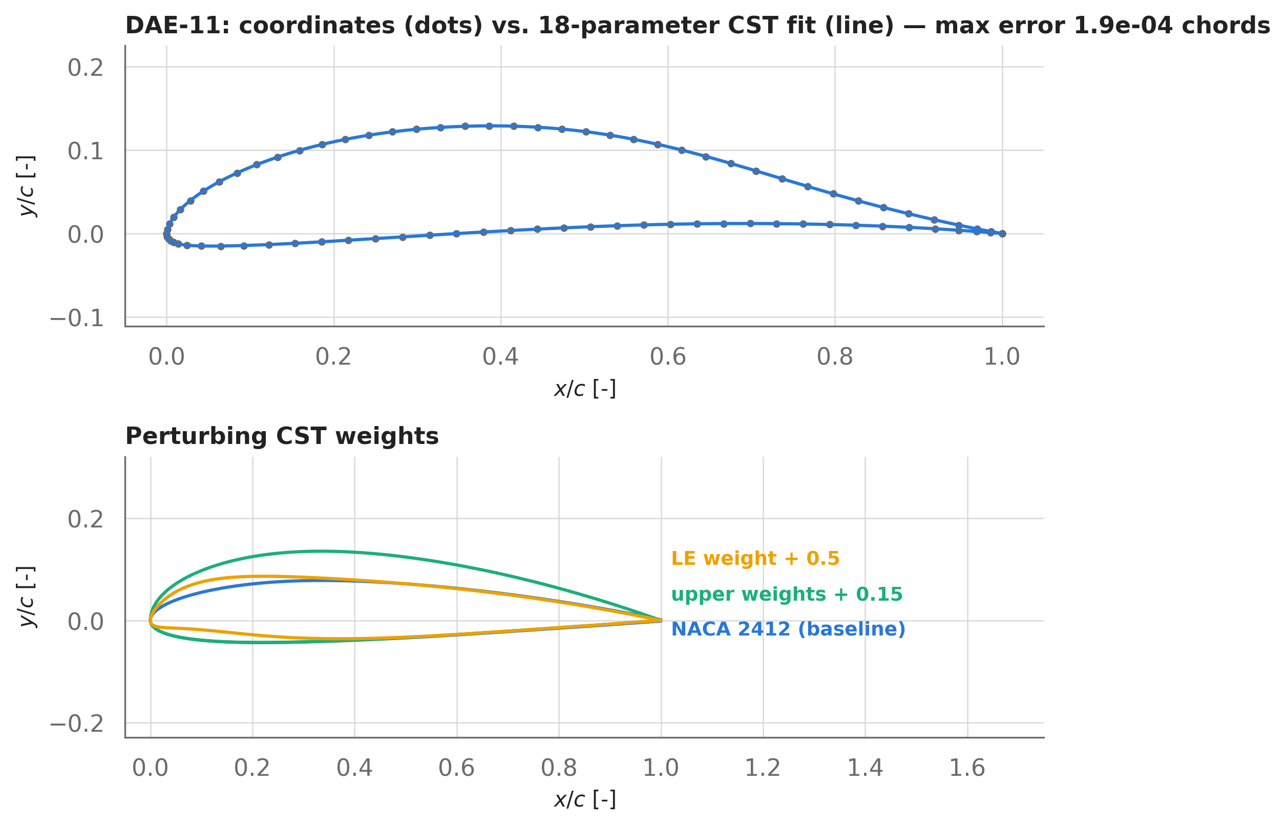
A KulfanAirfoil is a drop-in subclass of Airfoil — you can hand it to a WingXSec or query max_thickness() exactly as before. The payoff comes in optimization: because the shape is an analytic function of the weights, geometric quantities (and NeuralFoil’s aerodynamic predictions) are smooth, differentiable functions of the design variables. Airfoil shape optimization using exactly this parameterization is the flagship example of Chapter 6.
5.3 Wings
A wing in AeroSandbox is a stack of 2D slices. Each asb.WingXSec (“wing cross-section”) pins down one slice with four things: the leading-edge point xyz_le (in geometry axes), a chord, a twist angle (degrees, positive nose-up, applied about the leading edge), and an airfoil. The asb.Wing is the ordered root-to-tip list of these slices; between each adjacent pair, the surface is lofted linearly. So a wing with \(N\) cross-sections has \(N-1\) lofted sections — taper, sweep, and dihedral are not separate inputs but simply consequences of where you put the cross-sections and how big you make them.
One flag deserves special attention: symmetric=True tells AeroSandbox that you have defined only the right (\(+y\)) half, and the left half is its mirror image across the XZ plane. Main wings and horizontal tails are symmetric=True; a single centerline vertical fin is not.
Here is the main wing of our Cessna 152-class trainer. The real airplane’s dimensions are in feet and inches, so we convert at the boundary:
from aerosandbox.tools import units as u

def ft(feet, inches=0.0):
    """Convert feet-and-inches to meters."""
    return feet * u.foot + inches * u.inch

wing_airfoil = asb.Airfoil("naca2412")

wing = asb.Wing(
    name="Main Wing",
    symmetric=True,  # Define the right half; the left half is mirrored automatically.
    xsecs=[
        asb.WingXSec(  # Root, at the origin
            xyz_le=[0, 0, 0],
            chord=ft(5, 4),
            airfoil=wing_airfoil,
            control_surfaces=[
                asb.ControlSurface(name="Flap", symmetric=True, hinge_point=0.75)
            ],
        ),
        asb.WingXSec(  # Mid-span: constant chord so far, with 1 deg of dihedral
            xyz_le=[0, ft(7), ft(7) * np.sind(1)],
            chord=ft(5, 4),
            airfoil=wing_airfoil,
            control_surfaces=[
                asb.ControlSurface(name="Aileron", symmetric=False, hinge_point=0.75)
            ],
        ),
        asb.WingXSec(  # Tip: tapered and washed out, thinner section
            xyz_le=[
                ft(4, 0.75) - ft(3, 8.5),   # LE sweeps back as the chord shrinks
                ft(33, 4) / 2,               # half of the 33'4" span
                ft(33, 4) / 2 * np.sind(1),  # 1 deg dihedral, continued
            ],
            chord=ft(3, 8.5),
            twist=-1,  # washout, in degrees
            airfoil=asb.Airfoil("naca0012"),
        ),
    ],
)
wing
Wing 'Main Wing' (3 xsecs, symmetric)Two details of the definition above:
- Airfoils blend along the loft. The root and mid-span sections are NACA 2412; the tip is a NACA 0012. Analysis modules interpolate section properties between adjacent cross-sections, so the outboard panel smoothly transitions from cambered to symmetric.
- Twist is applied about an axis through each cross-section’s leading edge, directed along the (YZ-projected) line connecting adjacent quarter-chord points. Washout — negative twist at the tip, here −1° — is the classic trick to keep the tip flying below stall when the root stalls first.
5.3.1 Derived quantities
Once the cross-sections exist, every planform property an aero or structures model needs is a method call away — computed from the geometry itself, not entered separately (so they can never disagree with the geometry):
print(f"Span:            {wing.span():.3f} m")
print(f"Planform area:   {wing.area():.3f} m^2")
print(f"Wetted area:     {wing.area(type='wetted'):.3f} m^2")
print(f"Aspect ratio:    {wing.aspect_ratio():.3f}")
print(f"MAC:             {wing.mean_aerodynamic_chord():.3f} m")
print(f"Taper ratio:     {wing.taper_ratio():.3f}")
print(f"1/4-chord sweep: {wing.mean_sweep_angle():.2f} deg")
print(f"Dihedral:        {wing.mean_dihedral_angle():.2f} deg")
print(f"Aero center:     {wing.aerodynamic_center().round(3)} (geometry axes, m)")
Span: 10.162 m
Planform area: 15.059 m^2
Wetted area: 30.772 m^2
Aspect ratio: 6.857
MAC: 1.500 m
Taper ratio: 0.695
1/4-chord sweep: -0.18 deg
Dihedral: 1.06 deg
Aero center: [0.402 0. 0.043] (geometry axes, m)In words: the aspect ratio is the span squared over the planform area, \(A\!R = b^2/S\); the mean aerodynamic chord (MAC) is the chord-weighted average chord \(\bar{c} = \frac{2}{S}\int_0^{b/2} c^2\, \mathrm{d}y\), evaluated exactly per trapezoidal section; and the aerodynamic center is placed at quarter-MAC of each section, area-weighted. Note the wetted area is a bit more than twice the planform area — both surfaces, plus airfoil-thickness effects, via the airfoil’s perimeter().
import _common
import matplotlib.pyplot as plt

x_le = np.array([xsec.xyz_le[0] for xsec in wing.xsecs])
y_le = np.array([xsec.xyz_le[1] for xsec in wing.xsecs])
chords = np.array([xsec.chord for xsec in wing.xsecs])

fig, ax = plt.subplots(figsize=(8, 3.2))
for side in [+1, -1]:  # right half, then mirrored left half
    y = side * y_le
    outline_x = np.concatenate([x_le, (x_le + chords)[::-1], x_le[:1]])
    outline_y = np.concatenate([y, y[::-1], y[:1]])
    ax.fill(outline_y, outline_x, color=_common.GRID, alpha=0.5, zorder=1)
    ax.plot(outline_y, outline_x, color=_common.TEXT_PRIMARY, linewidth=1.2)
    ax.plot(y, x_le + 0.25 * chords, "--", color=_common.SERIES[0], linewidth=1.2)

ac = wing.aerodynamic_center()
ax.plot(ac[1], ac[0], "o", color=_common.SERIES[3], markersize=7, zorder=10)
ax.annotate("aerodynamic center", xy=(ac[1], ac[0]), xytext=(0.6, -0.55),
            color=_common.SERIES[3], fontweight="bold", fontsize=9,
            arrowprops=dict(arrowstyle="-", color=_common.SERIES[3], lw=0.8))
ax.annotate("quarter-chord line", xy=(3.2, x_le[1] + 0.25 * chords[1]),
            xytext=(2.2, -0.75), color=_common.SERIES[0], fontweight="bold",
            fontsize=9,
            arrowprops=dict(arrowstyle="-", color=_common.SERIES[0], lw=0.8))
ax.invert_yaxis()  # +x is aft, so flip to put the leading edge at the top
ax.set_aspect("equal", adjustable="datalim")
ax.set_xlabel("$y_g$ [m]")
ax.set_ylabel("$x_g$ [m]")
ax.set_title("Main wing planform")
plt.tight_layout()
plt.show()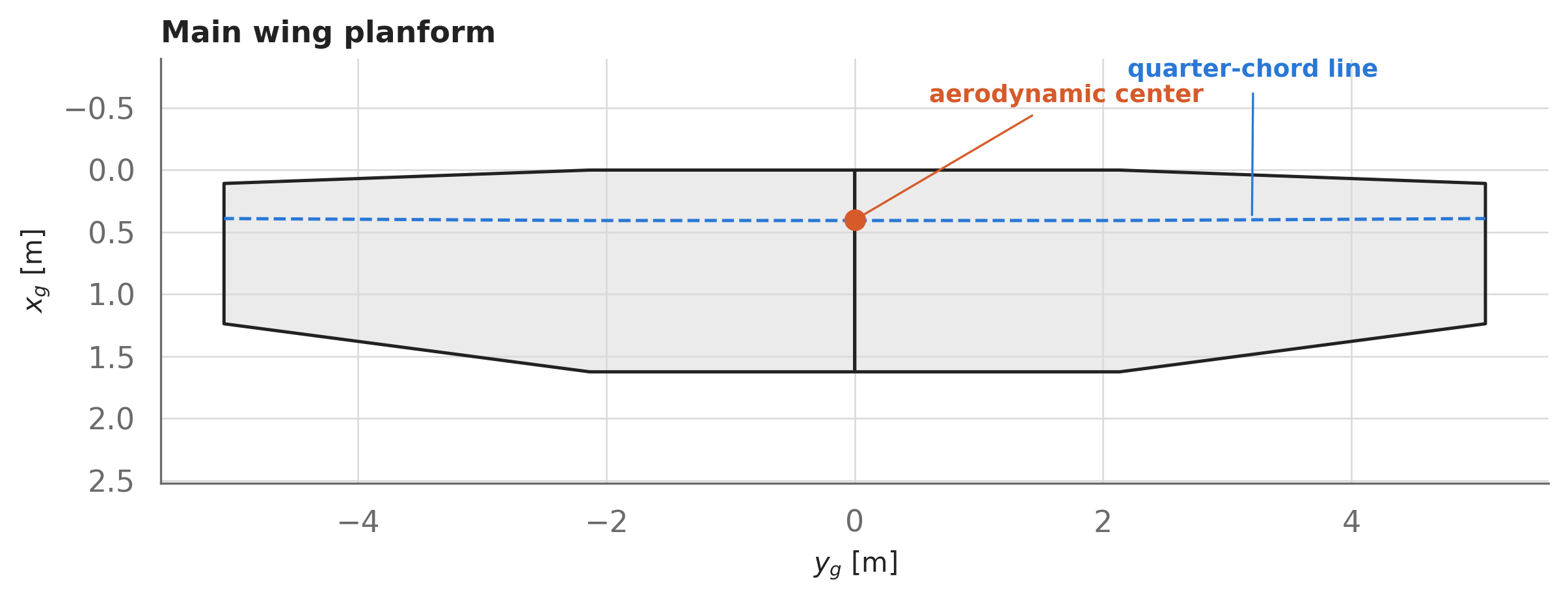
5.3.2 Control surfaces
Control surfaces are attached to a WingXSec via its control_surfaces list, and each asb.ControlSurface extends spanwise from that cross-section to the next one. In the wing above, the flap runs root → mid-span and the aileron runs mid-span → tip. Each surface has:
symmetric:Truemeans both sides deflect together (flaps, elevators);Falsemeans they deflect in opposition (ailerons), producing a rolling moment.hinge_point: hinge chordwise location as a fraction of local chord (0.75 here — the aft quarter of the chord is movable).deflection: in degrees, trailing-edge-down positive.
wing.get_control_surface_names()['Flap', 'Aileron']Deflections are just numbers on the geometry — set them directly, or use the name-based helpers:
wing.set_control_surface_deflections({"Flap": 10})  # degrees, in-place
print(f"Flap area: {wing.control_surface_area(by_name='Flap'):.2f} m^2 (both sides)")
Flap area: 1.73 m^2 (both sides)wing.set_control_surface_deflections({"Flap": 0}) # ...and back to clean configThe aerodynamics modules (Chapter 7) read these deflections when computing forces and moments. At the airplane level, airplane.with_control_deflections({...}) returns a deflected copy without mutating the original — convenient for sweeping elevator angles in a trim study.
5.4 Fuselages
Fuselages follow the same recipe as wings: an ordered list of cross-sections, lofted in sequence. An asb.FuselageXSec is a 2D shape on a plane, defined by a center point xyz_c, a size — either a radius, or a width and height — and a shape parameter. Cross-section planes default to facing along \(x\) but can be tilted via xyz_normal (useful for upswept tails and nacelle inlets).
The shape parameter deserves a picture. Fuselage cross-sections are superellipses: with half-width \(a\) and half-height \(b\), the perimeter satisfies
\[ \left|\frac{y}{a}\right|^{s} + \left|\frac{z}{b}\right|^{s} = 1, \]
so \(s = 2\) is an ellipse, \(s \to \infty\) approaches a rectangle, and \(s = 1\) is a diamond. Real aircraft cabins are usually somewhere between “round” and “square” — a single number captures that family:
import _common
import matplotlib.pyplot as plt

fig, ax = plt.subplots(figsize=(6, 4.2))
theta = np.linspace(0, 2 * np.pi, 361)
for s, color in zip([1, 1.5, 2, 4, 10], _common.SERIES):
    xsec = asb.FuselageXSec(xyz_c=[0, 0, 0], width=2, height=1.4, shape=s)
    x, y, z = xsec.get_3D_coordinates(theta=theta)
    ax.plot(y, z, color=color, linewidth=1.6)
    y45, z45 = np.interp(np.pi / 4, theta, y), np.interp(np.pi / 4, theta, z)
    _common.label_line(ax, y45, z45, f"shape={s}", color, dx=0.06, dy=0.05)
ax.set_aspect("equal", adjustable="datalim")
ax.set_xlabel("$y_g$ [m]")
ax.set_ylabel("$z_g$ [m]")
ax.set_title("FuselageXSec shapes: diamond (1) to ellipse (2) to squarish (10)")
plt.tight_layout()
plt.show()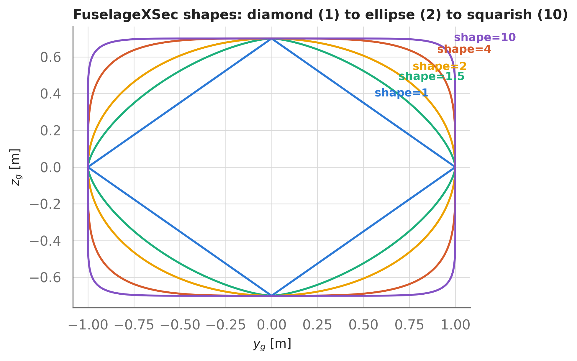
shape parameter, for a cross-section of width 2 m and height 1.4 m.
Our trainer’s fuselage takes six hand-placed stations — nose cap, cowl, windshield, cabin, and tail cone — with squarish (shape=3–4) sections through the cabin and round ones at the tail. The chained .translate() shifts the whole component so the nose sits ahead of and below the wing-root origin (it’s a high-wing airplane), and .subdivide_sections(2) inserts interpolated cross-sections into each loft segment for smoother drawing and meshing:
fuselage = asb.Fuselage(
    name="Fuselage",
    xsecs=[
        asb.FuselageXSec(xyz_c=[0, 0, ft(-1)], radius=0),  # nose point
        asb.FuselageXSec(xyz_c=[0, 0, ft(-1)], radius=ft(1.5), shape=4),  # cowl face
        asb.FuselageXSec(xyz_c=[ft(3), 0, ft(-0.85)], radius=ft(1.7), shape=4),
        asb.FuselageXSec(xyz_c=[ft(5), 0, 0], radius=ft(2.7), shape=3),  # cabin
        asb.FuselageXSec(xyz_c=[ft(10, 4), 0, ft(0.3)], radius=ft(2.3), shape=3),
        asb.FuselageXSec(xyz_c=[ft(21, 11), 0, ft(0.8)], radius=ft(0.3)),  # tail
    ],
).translate([ft(-5), 0, ft(-3)]).subdivide_sections(2)
fuselage
Fuselage 'Fuselage' (11 xsecs)(For smoothly-lofted bodies you can also generate stations programmatically — a favorite trick is radius=asb.Airfoil("naca0024").local_thickness(x_over_c=xi) swept over xi = np.cosspace(0, 1, 30), which produces a clean streamlined body of revolution from an airfoil’s thickness distribution.)
Like wings, fuselages know their derived quantities:
print(f"Length:         {fuselage.length():.3f} m")
print(f"Wetted area:    {fuselage.area_wetted():.3f} m^2")
print(f"Volume:         {fuselage.volume():.3f} m^3")
print(f"Fineness ratio: {fuselage.fineness_ratio():.2f}")
Length: 6.680 m
Wetted area: 23.583 m^2
Volume: 7.480 m^3
Fineness ratio: 5.59The fineness ratio (length over effective diameter) is the headline number here — it drives fuselage form drag and appears throughout the drag buildup in Chapter 7.
5.5 Propulsors
The asb.Propulsor is deliberately simple: a disk (length=0, the default) or a cylinder (length > 0), with a center xyz_c, an orientation xyz_normal (defaults to facing forward), and a radius. A disk is the right abstraction for a propeller or rotor — an actuator disk — while a cylinder roughly bounds a turbofan or ducted fan. Our trainer swings a 69-inch-diameter propeller at the nose:
propeller = asb.Propulsor(
    name="Propeller",
    xyz_c=[ft(-5.3), 0, ft(-4)],  # just ahead of the nose
    radius=ft(0, 34.5),           # 69-inch diameter
)
print(f"Disk area: {propeller.xsec_area():.3f} m^2")
Disk area: 2.412 m^2Disk area is the quantity you actually want downstream: actuator-disk theory converts it plus a thrust requirement into induced power (see the propulsion models in Chapter 9).
5.6 Assembling the Airplane
The asb.Airplane collects the components. We still need tail surfaces — a horizontal stabilizer (a symmetric wing with built-in negative incidence and an elevator) and a vertical fin (an asymmetric wing standing in the XZ plane, with a rudder):
tail_airfoil = asb.Airfoil("naca0012")

h_stab = asb.Wing(
    name="Horizontal Stabilizer",
    symmetric=True,
    xsecs=[
        asb.WingXSec(
            xyz_le=[0, 0, 0], chord=ft(3, 8), twist=-2, airfoil=tail_airfoil,
            control_surfaces=[
                asb.ControlSurface(name="Elevator", symmetric=True, hinge_point=0.75)
            ],
        ),
        asb.WingXSec(
            xyz_le=[ft(1), ft(5), 0], chord=ft(2, 4.375), twist=-2,
            airfoil=tail_airfoil,
        ),
    ],
).translate([ft(13, 3), 0, ft(-2)])

v_stab = asb.Wing(
    name="Vertical Stabilizer",  # no `symmetric` flag: a single centerline fin
    xsecs=[
        asb.WingXSec(xyz_le=[ft(-5), 0, 0], chord=ft(8, 8), airfoil=tail_airfoil),
        asb.WingXSec(
            xyz_le=[0, 0, ft(1)], chord=ft(3, 8), airfoil=tail_airfoil,
            control_surfaces=[
                asb.ControlSurface(name="Rudder", symmetric=True, hinge_point=0.75)
            ],
        ),
        asb.WingXSec(xyz_le=[ft(0, 8), 0, ft(5)], chord=ft(2, 8), airfoil=tail_airfoil),
    ],
).translate([ft(16, 11) - ft(3, 8), 0, ft(-2)])

airplane = asb.Airplane(
    name="Trainer (Cessna 152-like)",
    xyz_ref=[0.5, 0, -0.4],  # moment reference; we'll refine this to the true CG below
    wings=[wing, h_stab, v_stab],
    fuselages=[fuselage],
    propulsors=[propeller],
)
airplane
Airplane 'Trainer (Cessna 152-like)' (3 wings, 1 fuselage)The xyz_ref is the point about which analysis modules report moments — for it to mean anything physically, it should be the center of gravity (we compute one in Section 5.7 and update it there). If you don’t supply reference quantities, the Airplane derives them from the first wing in the list — which is why the main wing should come first:
print(f"s_ref = {airplane.s_ref:.3f} m^2   (first wing's planform area)")
print(f"c_ref = {airplane.c_ref:.3f} m     (first wing's mean aerodynamic chord)")
print(f"b_ref = {airplane.b_ref:.3f} m     (first wing's span)")
s_ref = 15.059 m^2 (first wing's planform area)
c_ref = 1.500 m (first wing's mean aerodynamic chord)
b_ref = 10.162 m (first wing's span)These are the normalizers behind every aerodynamic coefficient the library reports (\(C_L = L / (q_\infty S_\mathrm{ref})\), and so on). You can override any of them in the constructor — just be aware that reference-area conventions differ between organizations, so coefficients are only comparable when the references match.
Now the payoff — the drawing that catches 90% of geometry bugs:
axs = airplane.draw_three_view()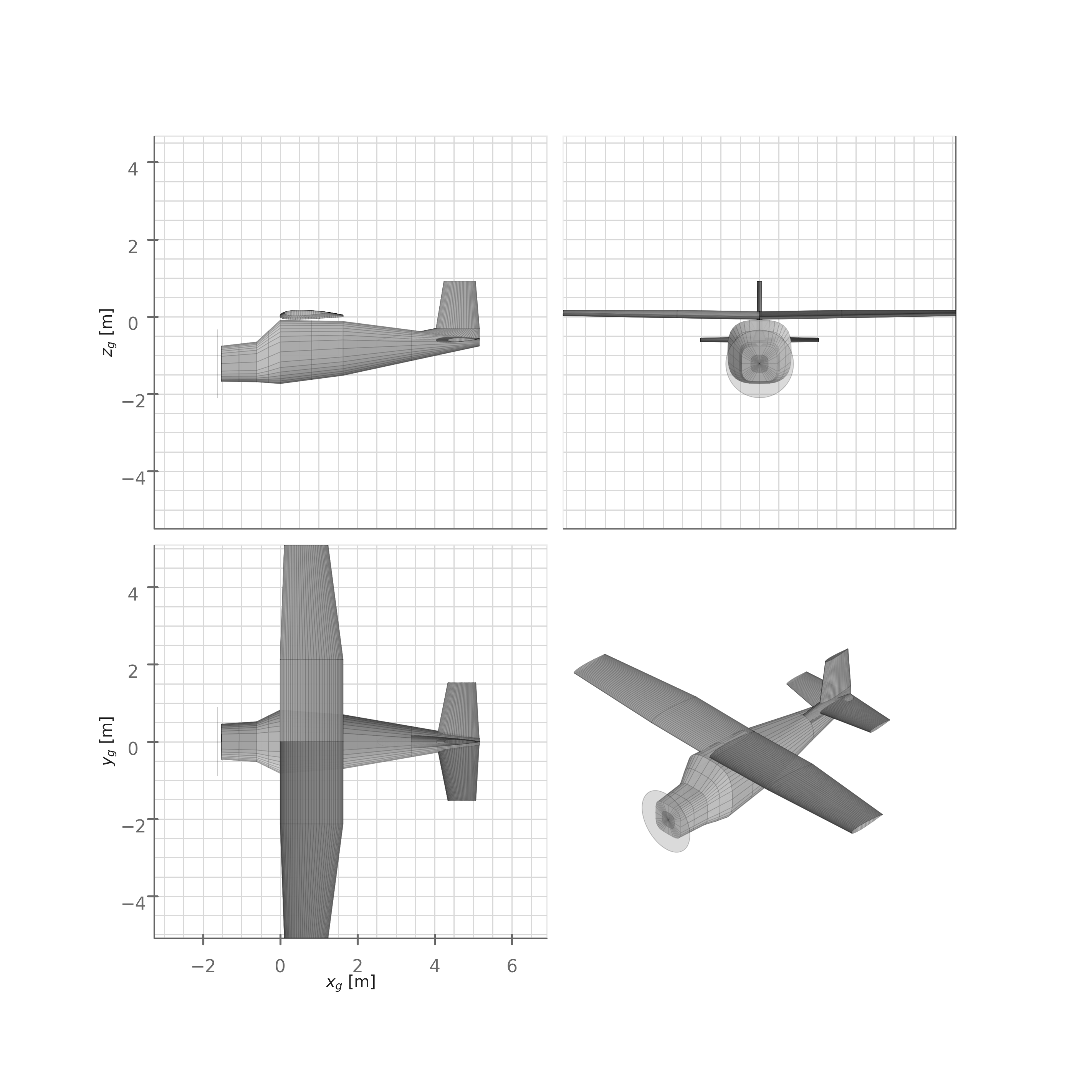
airplane.draw_three_view(): top, front, side, and isometric views, drawn with the Matplotlib backend. The translucent disk at the nose is the propeller.
Check it the way a designer reads a three-view: dihedral visible in the front view, high wing sitting atop the squarish cabin in the side view, taper starting at mid-span in the top view, propeller disk clear of the cowl. If you’d rather inspect the geometry interactively, airplane.draw() opens a 3D window (PyVista by default; backend="plotly" renders in-browser, and backend="matplotlib" accepts an ax= so you can compose it into your own figures — every draw method takes show=False if you want to annotate before displaying). A style="wireframe" option to draw_three_view() gives publication-style line drawings.
One more superpower of having geometry as data: it exports. airplane.export_AVL("trainer.avl") writes an AVL input file, export_XFLR5_xml(...) targets XFLR5, export_OpenVSP_vspscript(...) generates an OpenVSP script, and export_cadquery_geometry(...) produces a STEP file for CAD. Round-tripping to external tools is covered in Section 18.1.
5.6.1 Total wetted area
A quantity you will reach for constantly in drag estimation is the airplane’s total wetted area — and it falls straight out of the tree:
S_wet = (
    sum(w.area(type="wetted") for w in airplane.wings)
    + sum(f.area_wetted() for f in airplane.fuselages)
)
print(f"Total wetted area: {S_wet:.2f} m^2")
print(f"Wetted area ratio (S_wet / S_ref): {S_wet / airplane.s_ref:.2f}")
Total wetted area: 63.65 m^2
Wetted area ratio (S_wet / S_ref): 4.23That wetted-area ratio of 4.2 is the first number a designer computes when eyeballing parasite drag — Raymer’s classic \(C_{D_0} \approx C_{f_e} \, S_\mathrm{wet}/S_\mathrm{ref}\) estimate needs nothing else.
5.7 Mass properties
Geometry tells you where the air pushes; mass properties tell you how the airplane responds. The asb.MassProperties object bundles a mass, a center-of-gravity location, and an inertia tensor (about the CG, in whatever axes you defined the geometry — use geometry axes and be consistent). Its superpower is algebra: adding two MassProperties objects returns the properties of the combined rigid body, with the CG mass-averaged and the inertia tensors parallel-axis-shifted automatically. Multiplying by a scalar scales the mass. So a whole-vehicle weight buildup is literally sum(components.values()).
For quick component estimates, asb.mass_properties_from_radius_of_gyration() skips the tensor bookkeeping: give it a mass, a CG, and radii of gyration \(r\) about each axis, and it builds the diagonal inertia tensor \(I = m r^2\). Point masses need no radii at all. Here is a plausible buildup for our trainer (component masses in pounds-mass, from typical published data for this class of airplane; positions in geometry axes, eyeballed from the three-view):
b = wing.span()
L = fuselage.length()

components = {
    "Engine + propeller": asb.mass_properties_from_radius_of_gyration(
        mass=260 * u.lbm, x_cg=-1.15, z_cg=-0.55,  # up front, under the cowl
    ),
    "Wing": asb.mass_properties_from_radius_of_gyration(
        mass=230 * u.lbm, x_cg=0.85, z_cg=0.05,
        radius_of_gyration_x=b / 12**0.5,  # mass spread across the span...
        radius_of_gyration_z=b / 12**0.5,  # ...like a uniform rod, m*b^2/12
    ),
    "Fuselage + landing gear": asb.mass_properties_from_radius_of_gyration(
        mass=380 * u.lbm, x_cg=0.8, z_cg=-0.7,
        radius_of_gyration_y=L / 4, radius_of_gyration_z=L / 4,
    ),
    "Empennage": asb.mass_properties_from_radius_of_gyration(
        mass=55 * u.lbm, x_cg=4.4, z_cg=-0.2,
    ),
    "Systems + interior": asb.mass_properties_from_radius_of_gyration(
        mass=155 * u.lbm, x_cg=0.4, z_cg=-0.5,
    ),
    "Occupants (2)": asb.mass_properties_from_radius_of_gyration(
        mass=340 * u.lbm, x_cg=0.3, z_cg=-0.35,
    ),
    "Fuel": asb.mass_properties_from_radius_of_gyration(
        mass=160 * u.lbm, x_cg=0.85, z_cg=0.05,  # wing tanks
    ),
}

mass_props = sum(components.values())
mass_props
MassProperties instance:
Mass : 716.67594
Center of Gravity : ( 0.46993671, 0, -0.3778481)
Inertia Tensor :
(about CG) [ 953.42675, 0, -60.634965]
[ 0, 1280.397, 0]
[ -60.634965, 0, 2122.3764]The totals: 717 kg (1580 lbm) at takeoff, with the CG at \(x =\) 0.47 m. Notice what the algebra did for free: \(I_{xy} = I_{yz} = 0\) by left-right symmetry, but \(I_{xz} \neq 0\) — the engine hangs low and forward while the tail stretches aft and high, so the principal axes are slightly tilted from the body axes. That off-diagonal term is exactly what a 6-DOF dynamics simulation (Section 13.1) needs, and exactly what hand bookkeeping tends to drop. (If you need the tensor about a point other than the CG — say, a landing-gear pivot — use mass_props.get_inertia_tensor_about_point(...); for AVL’s .mass files there’s export_AVL_mass_file().)
import _common
import matplotlib.pyplot as plt
import aerosandbox.tools.pretty_plots as p

fig, ax = p.figure3d(figsize=(8, 4.5))
airplane.draw_wireframe(
    ax=ax, use_preset_view_angle="XZ", set_axis_visibility=False, show=False
)
for name, mp in components.items():
    ax.scatter([mp.x_cg], [0], [mp.z_cg],
               s=1.2 * mp.mass, color=_common.SERIES[0], alpha=0.6, zorder=100)
ax.scatter([mass_props.x_cg], [0], [mass_props.z_cg],
           s=150, color=_common.SERIES[3], marker="+", linewidth=3, zorder=101)
ax.text(mass_props.x_cg, 0, mass_props.z_cg - 0.6, "CG",
        color=_common.SERIES[3], ha="center", fontweight="bold", zorder=101)
ax.text(components["Engine + propeller"].x_cg, 0, 0.1, "engine",
        color=_common.SERIES[0], ha="center", fontsize=9, zorder=101)
ax.text(components["Empennage"].x_cg, 0, -1.45, "empennage",
        color=_common.SERIES[0], ha="center", fontsize=9, zorder=101)
plt.subplots_adjust(left=-0.6, right=1.6, bottom=-0.6, top=1.6)  # zoom in
plt.show()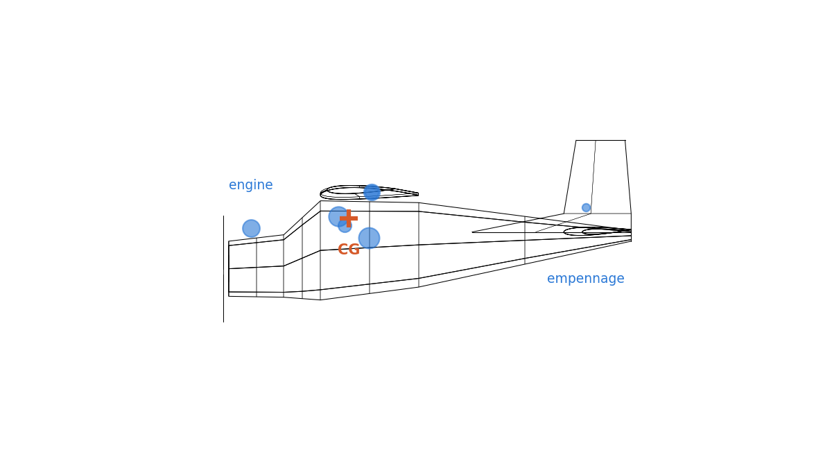
With a CG in hand, close the loop on the geometry — point the moment reference at it:
airplane.xyz_ref = mass_props.xyz_cgAs a sanity check, compare the CG against airplane.aerodynamic_center() — a purely geometric estimate of the neutral point that area-weights each lifting surface’s quarter-MAC:
x_np_geometric = airplane.aerodynamic_center()[0]
static_margin = (x_np_geometric - mass_props.x_cg) / airplane.c_ref
print(f"Geometric neutral-point estimate: x = {x_np_geometric:.2f} m")
print(f"CG:                               x = {mass_props.x_cg:.2f} m")
print(f"Static margin (geometric):        {static_margin:.1%} of MAC")
Geometric neutral-point estimate: x = 1.03 m
CG: x = 0.47 m
Static margin (geometric): 37.4% of MACThe CG lands ahead of the neutral point — statically stable, as it must be. Treat the magnitude with suspicion, though: this estimate credits the tail with its full area, ignoring downwash and the destabilizing fuselage, so it overstates the true static margin (here 37%; a real airplane of this type trims nearer 15–20%). The honest number comes from aerodynamic stability derivatives, computed in Chapter 7.
5.8 Geometry as optimization variables
Everything above used plain floats — but none of it had to. Any scalar in the geometry tree can be an Opti decision variable, and every derived quantity then becomes a symbolic, differentiable function of the design. A minimal (deliberately toy) demonstration — find the highest-aspect-ratio tapered wing that holds a fixed planform area within a span limit:
opti = asb.Opti()

span = opti.variable(init_guess=10, lower_bound=0)
root_chord = opti.variable(init_guess=1.5, lower_bound=0.2)

opt_wing = asb.Wing(
    symmetric=True,
    xsecs=[
        asb.WingXSec(xyz_le=[0, 0, 0], chord=root_chord, airfoil=wing_airfoil),
        asb.WingXSec(xyz_le=[0, span / 2, 0], chord=0.7 * root_chord,
                     airfoil=wing_airfoil),
    ],
)

opti.subject_to([
    opt_wing.area() == 15,  # m^2
    span <= 11,             # m
])
opti.minimize(-opt_wing.aspect_ratio())

sol = opti.solve(verbose=False)
opt_wing = sol(opt_wing)  # substitute the solution back into the geometry object

print(f"Optimal span:  {sol(span):.2f} m   (hits the constraint, as expected)")
print(f"Root chord:    {sol(root_chord):.3f} m")
print(f"Aspect ratio:  {opt_wing.aspect_ratio():.2f}")
Optimal span: 11.00 m (hits the constraint, as expected)
Root chord: 1.604 m
Aspect ratio: 8.07Note the last trick: sol(opt_wing) recursively substitutes the solved values through the entire object, returning a concrete Wing you can draw, mesh, or export. The same pattern scales to a full Airplane with hundreds of geometric design variables — that, plus aerodynamic and structural models pushing back against each other, is the substance of Chapter 10 and the design studies in later chapters.
5.9 Where to go next
- Chapter 6 puts the
AirfoilandKulfanAirfoilobjects to work: NeuralFoil polars, and airfoil shape optimization directly in the CST parameter space. - Chapter 7 feeds the
Airplanewe just built into the 3D analysis ladder —AeroBuildup, vortex-lattice, and stability derivatives that replace this chapter’s geometric static-margin estimate with the real thing. - Chapter 10 begins design optimization in earnest, where the geometry’s chords and spans stop being numbers and become the unknowns.