flowchart TD
    A["opti.solve() failed"] --> B{"read the<br/>return_status"}
    B -->|"Invalid_Number_Detected"| C{"failed at<br/>iteration 0?"}
    C -->|"yes"| D["NaN at the initial guess.<br/>Evaluate the model at the guess<br/>and fix the guess or the domain."]
    C -->|"no"| E["An iterate left a function's domain<br/>(sqrt, log, arcsin, division).<br/>Add domain guards or log-transform."]
    B -->|"Infeasible_Problem_Detected"| F["Constraints conflict.<br/>Run sol.show_infeasibilities()<br/>and relax one at a time."]
    B -->|"Diverging_Iterates"| G["Problem is unbounded:<br/>nothing pushes back on the objective.<br/>Add the missing physics or bounds."]
    B -->|"Maximum_Iterations_Exceeded"| H["Usually poor scaling.<br/>Set scale= on every variable;<br/>check for zero initial guesses."]
    B -->|"Restoration_Failed /<br/>Error_In_Step_Computation"| I["Kink or non-smoothness<br/>near the optimum.<br/>Smooth or reformulate it."]
Appendix B — FAQ and Troubleshooting
This appendix is where you come when something breaks. It gives you a decision tree for diagnosing a failed solve from its IPOPT exit code, a forensic workflow (opti.debug) for interrogating the last iterate of a failed optimization, a decoder table for the solver statuses you’ll actually encounter, performance guidance for when a solve is working but slow, and short answers to the questions most often asked on the AeroSandbox issue tracker. Every failure mode shown here is reproduced live in this document — the error messages and exit codes you see below are real output from the current library, not paraphrases.
B.1 First response to a failed solve
When opti.solve() fails, it does not fail silently — it tells you how it failed, via IPOPT’s return status. Reading that status is always the first move, because each status points to a different class of bug and a different fix. You can find it in three places:
- In the exception message. A failed solve raises a
RuntimeErrorwhose text ends with something likereturn_status is 'Infeasible_Problem_Detected'. - In
opti.debug.stats()["return_status"], available after the exception is raised. - In
sol.stats()["return_status"], if you solved withbehavior_on_failure="return_last"— which suppresses the exception and hands you the last iterate wrapped as a normal solution object.
With the status in hand, the diagnosis is nearly mechanical:
The chapters on robust optimization models and solvers teach how to avoid each of these failures; this appendix focuses on recognizing and dissecting them after the fact.
B.1.1 The failure zoo, reproduced live
To make the decision tree concrete, here are the four canonical failures as minimal problems — each engineered to fail in exactly one way. The helper solves each with behavior_on_failure="return_last" so we can collect the exit statuses instead of catching exceptions:
import aerosandbox as asb
import aerosandbox.numpy as np
import warnings


def status_of(build_problem, **solve_kwargs) -> str:
    """Build a problem, attempt to solve it, and report IPOPT's return status."""
    opti = asb.Opti()
    build_problem(opti)
    with warnings.catch_warnings():
        warnings.simplefilter("ignore")  # silence the "solve failed" UserWarning
        sol = opti.solve(verbose=False, behavior_on_failure="return_last", **solve_kwargs)
    return sol.stats()["return_status"]


def infeasible(opti):  # two constraints that cannot both hold
    x = opti.variable(init_guess=0)
    opti.subject_to([x >= 2, x <= 1])
    opti.minimize(x**2)


def unbounded(opti):  # nothing pushes back on the objective
    x = opti.variable(init_guess=0)
    opti.minimize(-x)


def nan_at_start(opti):  # initial guess outside the model's domain
    x = opti.variable(init_guess=-1)
    opti.minimize(np.sqrt(x))


def kinked(opti):  # |x| built as sqrt(x^2): no derivative at the optimum
    x = opti.variable(init_guess=1)
    opti.minimize(np.sqrt(x**2))


statuses = {f.__name__: status_of(f) for f in [infeasible, unbounded, nan_at_start, kinked]}

for name, status in statuses.items():
    print(f"{name:14s} -> {status}")
infeasible -> Infeasible_Problem_Detected
unbounded -> Diverging_Iterates
nan_at_start -> Invalid_Number_Detected
kinked -> Error_In_Step_ComputationEach toy maps onto a real modeling bug you will eventually write. The infeasible case is a stall-speed requirement fighting a span limit. The unbounded case is a drag-minimization with no weight model — the optimizer happily drives wing area to zero or aspect ratio to infinity, and Diverging_Iterates is IPOPT noticing the iterates running off to infinity (the wing design chapter dissects a subtler version of this disease, where the problem is bounded but the answer is nonsense — see Section 10.5). The nan_at_start case is any sqrt, log, or arcsin fed an out-of-domain value by your initial guesses. And kinked is an absolute value, a np.maximum, or a table lookup with a slope discontinuity sitting exactly where the optimizer wants to converge.
B.1.2 The fifth failure: scaling
Maximum_Iterations_Exceeded deserves its own demonstration, because it is the most common failure on real problems and the least informative-sounding. It usually does not mean “the problem is too hard” — it means the problem is badly scaled, so IPOPT limps toward the optimum in tiny, ill-conditioned steps until the budget runs out. Here is a problem whose two variables have optima 12 orders of magnitude apart. We give the solver the same 20-iteration budget twice — first with no scale information, then with scale= hints:
def make_mismatched_problem(use_scale: bool):
    opti = asb.Opti()
    x = opti.variable(init_guess=1, scale=1e-6 if use_scale else None)  # optimum near 1e-6
    y = opti.variable(init_guess=1, scale=1e6 if use_scale else None)  # optimum near 1e+6
    opti.subject_to(x * y >= 1)
    opti.minimize((1e6 * x - 1) ** 2 + (1e-6 * y - 1) ** 2)
    return opti


with warnings.catch_warnings():
    warnings.simplefilter("ignore")
    sol_unscaled = make_mismatched_problem(use_scale=False).solve(
        verbose=False, max_iter=20, behavior_on_failure="return_last"
    )
    sol_scaled = make_mismatched_problem(use_scale=True).solve(
        verbose=False, max_iter=20, behavior_on_failure="return_last"
    )

for name, sol in [("no scale info", sol_unscaled), ("with scale=", sol_scaled)]:
    print(
        f"{name:14s} -> {sol.stats()['return_status']:28s} "
        f"({sol.stats()['iter_count']} iterations)"
    )
no scale info -> Maximum_Iterations_Exceeded (20 iterations)
with scale= -> Solve_Succeeded (5 iterations)Same physics, same budget: the version without scale information runs out of budget, while the scaled one converges in 5 iterations. On this toy, IPOPT would eventually recover if given more iterations; on a thousand-variable aircraft model it often will not. The full theory and a dramatic real-world example (an order-of-magnitude speedup on a rocket trajectory) are in Section 3.4.
B.2 The opti.debug workflow
The most important debugging fact about a failed solve: the last iterate is always available, even though no solution exists. Where the optimizer got stuck is usually a giant arrow pointing at the modeling bug. Here is the full forensic loop on a small wing-sizing problem that is subtly overconstrained — a stall-speed requirement, a hangar-width span limit, and an aspect-ratio floor that cannot all coexist:
opti = asb.Opti()

S = opti.variable(init_guess=12, scale=10)  # wing area [m^2]
b = opti.variable(init_guess=10, scale=10)  # wingspan [m]

V_stall = opti.parameter(value=25)  # required stall speed [m/s]

mass = 600  # aircraft mass [kg]
CL_max = 1.5  # max lift coefficient [-]

opti.subject_to(
    0.5 * 1.225 * V_stall**2 * S * CL_max >= mass * 9.81  # can lift weight at stall
)
opti.subject_to(b <= 12)  # span limit: must fit in the hangar
opti.subject_to(b**2 / S >= 15)  # aspect ratio floor, for induced drag

opti.minimize(S)  # wetted-area (drag, weight, cost) proxy

try:
    sol = opti.solve(verbose=False)
except RuntimeError as e:
    print(f"{type(e).__name__}: ...{str(e)[-120:]}")
RuntimeError: ...u may use opti.debug.value to investigate the latest values of variables. return_status is 'Infeasible_Problem_Detected'The exception message itself tells you the status and the next move: opti.debug. After a raised failure, opti.debug.value() evaluates any expression — variables, or functions of them — at the last iterate:
print(f"Last iterate:  S = {opti.debug.value(S):.2f} m^2,  b = {opti.debug.value(b):.2f} m")
print(f"Aspect ratio there:  b^2/S = {opti.debug.value(b**2 / S):.2f}")
Last iterate: S = 10.25 m^2, b = 12.40 m
Aspect ratio there: b^2/S = 15.00The story is already legible: the last iterate sits at the stall-bound wing area with the aspect ratio pinned exactly at its floor — and to manage both at once, the solver had to stretch the span to 12.4 m, 0.4 m more than the hangar allows. The three constraints form a loop with no slack anywhere. To get the diagnosis spelled out — every violated constraint, with the source line in your code that created it — re-solve with behavior_on_failure="return_last" and call sol.show_infeasibilities():
with warnings.catch_warnings():
    warnings.simplefilter("ignore")
    sol = opti.solve(verbose=False, behavior_on_failure="return_last")

sol.show_infeasibilities(tol=1e-3)
--------------------------------------------------
12.399868209734413 < 12.0 (violation: 0.3998682097344126)
Scalar constraint defined in `945354852.py`, line 14:
```
opti.subject_to(b <= 12) # span limit: must fit in the hangar
```From here the resolution is an engineering decision, not a numerical one: accept a faster stall speed, a wider hangar, or a stubbier wing. Because we declared V_stall as an opti.parameter(), testing the first option doesn’t even require rebuilding the problem:
sol = opti.solve(parameter_mapping={V_stall: 27}, verbose=False)

print(f"status: {sol.stats()['return_status']}")
print(f"S = {sol(S):.2f} m^2,  b = {sol(b):.2f} m,  AR = {sol(b**2 / S):.2f}")
status: Solve_Succeeded
S = 8.79 m^2, b = 11.74 m, AR = 15.69Two m/s of stall speed buys the design back. (For what a converged solution can tell you about which constraint to relax — the shadow price of each, for free — see Section 5.4.)
B.2.1 NaN forensics: evaluating the model at the initial guess
When the status is Invalid_Number_Detected at iteration 0, the model is producing NaN at your initial guesses, before the optimizer has taken a single step. You can hunt the NaN down without solving anything: opti.debug.value(expr, opti.initial()) evaluates any expression at the initial guess. Scan your intermediate quantities and find the first one that goes bad.
Here’s a climb-performance model with a classic domain bug — the steady-climb-angle formula \(\gamma = \arcsin\left((T - D)/W\right)\), evaluated at a flight condition where thrust exceeds drag plus weight, so the arcsine’s argument leaves \([-1, 1]\):
opti = asb.Opti()

V = opti.variable(init_guess=18, scale=10)  # airspeed [m/s]

W = 1200  # weight [N]
T = 1500  # thrust [N] (a very overpowered airplane)

q = 0.5 * 1.225 * V**2  # dynamic pressure [Pa]
D = q * 0.7 * 0.030  # drag [N]
sin_gamma = (T - D) / W  # sine of climb angle [-]
gamma = np.arcsin(sin_gamma)  # climb angle [rad]

opti.subject_to(V >= 15)
opti.maximize(gamma * V)  # rate of climb

with warnings.catch_warnings():
    warnings.simplefilter("ignore")
    sol = opti.solve(verbose=False, behavior_on_failure="return_last")

print(f"status: {sol.stats()['return_status']}  (at iteration {sol.stats()['iter_count']})")
status: Invalid_Number_Detected (at iteration 0)Now the hunt — evaluate each intermediate expression at the initial guess and look for the first NaN:
for name, expr in {"q": q, "D": D, "sin_gamma": sin_gamma, "gamma": gamma}.items():
    print(f"{name:10s} = {opti.debug.value(expr, opti.initial()):.4f}")
q = 198.4500
D = 4.1674
sin_gamma = 1.2465
gamma = nansin_gamma is fine as a number but out of range as an arcsine argument — and everything downstream of gamma is NaN. The bug isn’t numerical, it’s physical: the steady-climb formula assumes thrust small enough that the airplane can’t climb vertically, and this airplane violates that. The fix is to reformulate (e.g., treat \(\sin\gamma\) itself as the state, or constrain the argument away from the domain edge) — the systematic patterns are in Section 3.3.
B.3 IPOPT return codes, decoded
The statuses below cover essentially every exit you will see in practice. The first column is the exact string in sol.stats()["return_status"] (the four canonical failures were captured live in Section B.1.1).
return_status |
What IPOPT is telling you | Most likely cause in a design problem | First fix |
|---|---|---|---|
Solve_Succeeded |
Converged to tolerance. | — | Sanity-check the design anyway (Section 10.5). |
Solved_To_Acceptable_Level |
Progress stalled, but at a point meeting IPOPT’s looser “acceptable” tolerances. | Mild scaling or smoothness issues near the optimum. | Usually usable. To reach full tolerance, improve scaling (Section 3.4). |
Infeasible_Problem_Detected |
Converged — to a point that minimizes constraint violation, not your objective. | Genuinely conflicting requirements (or ones that only conflict through bad scaling). | sol.show_infeasibilities(); relax constraints one at a time (Section B.2). |
Maximum_Iterations_Exceeded |
Ran out of the iteration budget (max_iter, default 1000). |
Poor scaling, in ~90% of sightings. | scale= on every variable; honest initial guesses; log_transform=True for positive quantities. |
Maximum_CpuTime_Exceeded |
Ran out of wall-clock budget (max_runtime). |
Same as above, or a genuinely large problem. | Same as above; also see Section B.4. |
Diverging_Iterates |
Iterates ran off toward infinity. | Unbounded problem: the objective rewards something no constraint limits. | Add the missing physics — weight, stall, structure (Section 10.5). |
Invalid_Number_Detected |
NaN/Inf in the objective, constraints, or their derivatives. | Out-of-domain sqrt/log/arcsin/division — at iteration 0, blame the initial guess. |
NaN forensics (Section B.2.1); domain guards (Section 3.3). |
Restoration_Failed |
The feasibility-restoration fallback itself failed. | Non-smoothness or NaN-adjacent model regions near the iterate. | Smooth kinks (Section 3.2); buffer domain edges. |
Error_In_Step_Computation |
Could not compute a search step, typically near an apparent optimum. | A kink or infinite curvature exactly where the solution wants to be. | Epigraph reformulation or np.softmax smoothing (Section 3.2). |
Search_Direction_Becomes_Too_Small |
Steps shrank to numerical dust before tolerances were met. | Severe ill-conditioning / scaling. | Rescale variables and objective to order 1. |
Not_Enough_Degrees_Of_Freedom |
More equality constraints than free variables. | A modeling slip — e.g., freezing variables while keeping constraints that pinned them. | Recount your equalities; check what you froze. |
Two of these deserve a special warning. Solved_To_Acceptable_Level is a soft success — the answer is usually fine for conceptual design, but treat it as a nudge to fix your scaling before trusting sensitivities. And a plain Solve_Succeeded is a statement about the math, not the model: the optimizer found a local optimum of the problem you wrote down, which is not necessarily the problem you meant.
B.4 Performance: when the solve works but crawls
The single most common performance mistake in AeroSandbox is building vector quantities one scalar at a time in a Python loop — declaring \(N\) separate scalar variables instead of one vector variable, and adding \(N\) separate scalar constraints instead of one vectorized constraint. The optimizer sees the identical mathematical problem either way; what explodes is the bookkeeping. Every call to opti.variable() and opti.subject_to() does Python-side work (including inspecting the call stack, so that sol.show_infeasibilities() can later point at your source line), and every scalar operation adds its own node to CasADi’s computational graph — whereas one vectorized operation is a single node.
Here is the same trajectory-flavored problem — minimize distance to a wavy target profile, subject to a rate limit between adjacent points — built both ways, timed as problem size grows:
import time


def solve_scalar_loop(N: int):
    opti = asb.Opti()
    x = [opti.variable(init_guess=1) for _ in range(N)]  # N separate scalar variables
    for i in range(N - 1):
        opti.subject_to(x[i + 1] - x[i] <= 0.1)  # N-1 separate scalar constraints
    opti.minimize(sum((x[i] - np.sin(i)) ** 2 for i in range(N)))
    return opti.solve(verbose=False)


def solve_vectorized(N: int):
    opti = asb.Opti()
    x = opti.variable(init_guess=np.ones(N))  # one vector variable
    opti.subject_to(np.diff(x) <= 0.1)  # one vectorized constraint
    opti.minimize(np.sum((x - np.sin(np.arange(N))) ** 2))
    return opti.solve(verbose=False)


solve_vectorized(10)  # warm-up, so one-time library initialization doesn't skew timings

N_sweep = [10, 30, 100, 300, 1000]
t_loop, t_vec = [], []
for N in N_sweep:
    t0 = time.perf_counter()
    solve_scalar_loop(N)
    t1 = time.perf_counter()
    solve_vectorized(N)
    t2 = time.perf_counter()
    t_loop.append(t1 - t0)
    t_vec.append(t2 - t1)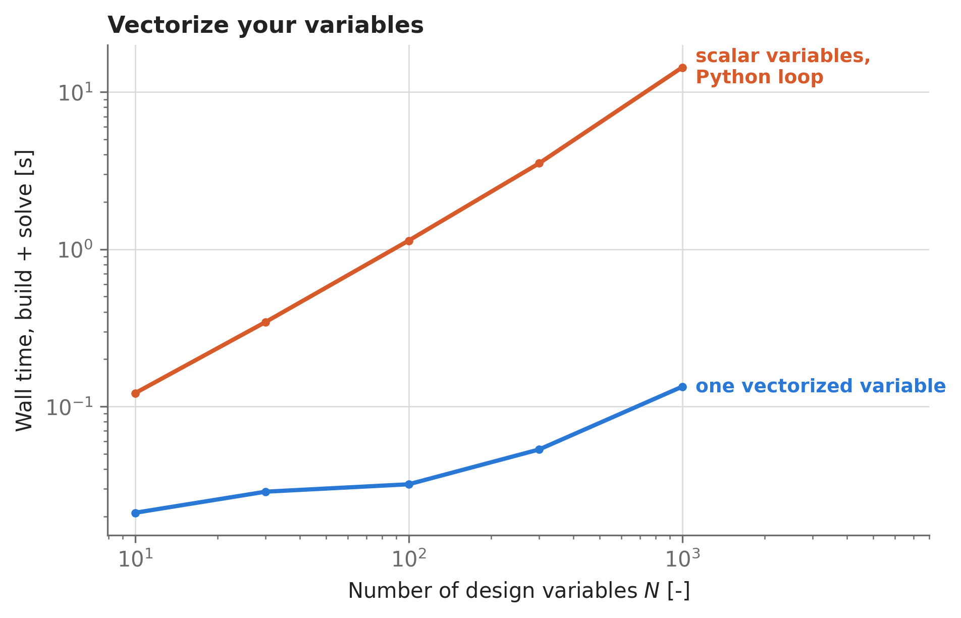
At \(N =\) 1000 variables, the vectorized formulation is 107× faster end-to-end — and the gap keeps widening with \(N\). A checklist for slow solves:
- Vectorize. One
opti.variable(init_guess=..., n_vars=N)per physical quantity, array operations fromaerosandbox.numpyfor the model, and vector constraints (opti.subject_to(np.diff(x) <= 0.1)rather than a loop). This is the same idiom the optimal control chapter uses for entire trajectories. - Scale. A poorly scaled problem that converges in 200 iterations instead of 20 is a 10× slowdown wearing a disguise (Section 3.4).
- Don’t rebuild the problem to change a number. If you re-solve while varying an input, declare it with
opti.parameter()and re-solve withparameter_mapping=— or useopti.solve_sweep(), which also supports warm-starting each solve from the previous one (Section 5.5). - Check where time actually goes.
sol.stats()reports evaluation counts and per-function times (n_call_nlp_f,t_wall_nlp_hess_l, …). If Hessian evaluations dominate, your model graph is heavy; if iteration count is huge, it’s scaling.
B.5 Frequently asked questions
B.5.1 Why do I have to use aerosandbox.numpy instead of regular NumPy?
Because your model must evaluate on two kinds of inputs: ordinary floats/arrays, and the symbolic CasADi objects that opti.variable() returns (that symbolic trace is where the exact derivatives come from — see Section 2.5). Plain NumPy doesn’t know about the symbolic type. Confusingly, some plain-NumPy functions happen to work on symbolics and others fail with cryptic errors:
import numpy as plain_np

opti = asb.Opti()
x = opti.variable(init_guess=1)

print(type(plain_np.sin(x)))  # happens to work (dispatches to CasADi)

try:
    plain_np.where(x > 1, x, 0)  # does not
except Exception as e:
    print(f"{type(e).__name__}: {e}")

print(type(np.where(x > 1, x, 0)))  # aerosandbox.numpy: works
<class 'casadi.casadi.MX'>
ValueError: setting an array element with a sequence.
<class 'casadi.casadi.MX'>aerosandbox.numpy re-exports everything from NumPy and overrides the functions that need dual-backend handling: on normal arrays it is NumPy (identical results, identical speed), and on symbolics it dispatches to the CasADi equivalent. So the rule is simply: import aerosandbox.numpy as np, always, and write your models once. If you hit a function that isn’t yet supported on symbolics, you’ll get an immediate TypeError/NotImplementedError — open an issue, as coverage grows by request.
B.5.2 Why can’t I use if statements on an optimization variable?
Because until the problem is solved, a variable has no value — so x > 3 is a symbolic expression, not a True/False. Python’s if, and, or, and while all demand an immediate boolean, and CasADi refuses:
opti = asb.Opti()
x = opti.variable(init_guess=1)

try:
    if x > 3:
        y = 0
except RuntimeError as e:
    print(f"RuntimeError: ...{str(e)[-60:]}")
RuntimeError: ...ode.cpp:203: Can only determine truth value of a numeric MX.The branching must instead live inside the computational graph, so the optimizer can differentiate through it: use np.where(condition, value_if_true, value_if_false), or better, the smooth blends np.blend() and np.softmax(). Beware that np.where introduces a kink (a slope discontinuity) at the switch point, which can produce exactly the Error_In_Step_Computation failures cataloged above if the optimum lands on it — Section 3.2 covers the smooth alternatives.
B.5.3 Does the initial guess really matter?
Yes, three times over. First, these are nonconvex problems: the initial guess selects which basin of attraction you converge into. Second, if you don’t pass scale=, the initial guess doubles as the variable’s scale — so init_guess=0 silently degrades scaling (the heuristic falls back to 1). Third, the model must be NaN-free at the guess, or you fail at iteration 0 (Section B.2.1). If you omit it entirely, AeroSandbox warns you and guesses 0:
with warnings.catch_warnings(record=True) as caught:
    warnings.simplefilter("always")
    x = asb.Opti().variable()
print(caught[0].message)
No initial guess set for Opti.variable(). Defaulting to 0.An honest, physical initial guess — the number you’d sketch on a napkin — is the cheapest solver acceleration available.
B.5.4 How do I get results out of a solution — and feed them back in?
Call the solution like a function. sol(expr) evaluates any expression at the optimum — single variables, derived quantities you never declared, or whole containers at once:
opti = asb.Opti()
x = opti.variable(init_guess=1)
y = opti.variable(init_guess=np.ones(3))
opti.minimize((x - 3) ** 2 + np.sum((y - 1) ** 2))
sol = opti.solve(verbose=False)

print(sol({"x": x, "y": y, "derived": x * 2 + np.mean(y)}))
{'x': 3.0, 'y': array([1., 1., 1.]), 'derived': 7.0}To feed a solution back in as the starting point of another solve — a warm start — use opti.set_initial_from_sol(sol). This is what makes parameter sweeps fast and reliable, since each solve starts from its neighbor’s answer; opti.solve_sweep(..., update_initial_guesses_between_solves=True) automates the whole pattern (Section 5.5).
B.5.5 Do I need to supply gradients or Hessians?
No — and you can’t do better than what you already get. Because your model is traced symbolically through aerosandbox.numpy, CasADi automatically generates exact first and second derivatives (sparse Jacobians and Hessians) via automatic differentiation, and IPOPT consumes them directly. You can see this in any solve’s statistics — the solver is calling an auto-generated exact Hessian, with zero user code:
print(f"Objective evaluations:      {sol.stats()['n_call_nlp_f']}")
print(f"Exact Hessian evaluations:  {sol.stats()['n_call_nlp_hess_l']}")
Objective evaluations: 2
Exact Hessian evaluations: 1This is precisely why non-traceable code (a Fortran executable, arbitrary scipy routines) can’t go directly inside the model — which brings us to the next question.
B.5.6 Can I optimize through XFoil, AVL, or my own external solver?
Not directly. AeroSandbox’s XFoil and AVL classes drive the real executables through files and subprocesses — invaluable for validation, but opaque to the derivative trace: the optimizer can’t see inside them. Three escape hatches, in order of preference:
- Use the native differentiable equivalent: NeuralFoil (Section 6.1) instead of XFoil,
AeroBuilduporVortexLatticeMethod(Section 7.3) instead of AVL. These were built for exactly this purpose. - Fit a surrogate: run the external tool offline over a grid, then optimize through a
FittedModelorInterpolatedModel(Section 17.3). - Wrap it with
asb.black_box, which exposes any Python-callable to the optimizer using finite differences (Section 17.4) — with all the noise and cost caveats that finite differencing implies.
The external tools chapter covers running XFoil/AVL/MSES from AeroSandbox for the validation role they’re best at.
B.5.7 How do I freeze design variables for an off-design study?
Once parts of a design are locked in (a built wing, an ordered engine), re-optimize the rest by freezing variables: opti.variable(..., freeze=True) pins one variable at its init_guess, and category-based freezing pins whole groups without touching the model code:
opti = asb.Opti(variable_categories_to_freeze=["geometry"])

span = opti.variable(init_guess=10, category="geometry")  # frozen at 10
V = opti.variable(init_guess=30, category="operations")  # still free

opti.minimize((span * V - 400) ** 2)
sol = opti.solve(verbose=False)
print(f"span = {sol(span):.1f} m (frozen),  V = {sol(V):.1f} m/s (optimized)")
span = 10.0 m (frozen), V = 40.0 m/s (optimized)The same machinery supports saving a solved design to a JSON cache (save_to_cache_on_solve=True) and later reloading the frozen values from that file (load_frozen_variables_from_cache=True) — see the asb.Opti.__init__ and Opti.variable docstrings for the full pattern. One trap worth knowing: if freezing makes some constraint contain no free variables at all and that constraint is violated, subject_to() raises immediately (the problem is infeasible as written); pass ignore_violated_parametric_constraints=True to skip such constraints instead.
B.5.8 My solve succeeded, but the design looks absurd. Is that a bug?
Almost certainly not a bug — a missing model. An optimizer is an adversary that exploits every effect you left out: minimize drag without a weight model and it returns a wing of near-infinite aspect ratio; maximize range without a structural model and it fills the wings with infinite fuel. Solve_Succeeded certifies a local optimum of the problem you wrote, nothing more. The wing design chapter walks through a complete post-mortem of one of these (Section 10.3) and the design principle that prevents them: every variable the optimizer can push must have a model that eventually pushes back (Section 10.5).
B.5.9 Something’s broken at install or import time
The essentials, most-common first:
- Install with
pip install aerosandbox[full]— the[full]extra adds interactive 3D visualization and geometry export (plotly, pyvista, trimesh, cadquery, …). A barepip install aerosandboxgives you the core numerics only. - Python version: 3.10 or newer is required (per the package metadata; older interpreters will fail at install-resolution time).
- Check your version when reporting anything — this document was executed against:
print(asb.__version__)4.2.9- “xfoil not found”-type errors: XFoil and AVL are not bundled with AeroSandbox and aren’t on your PATH by default. Either add them to PATH, or pass an explicit executable path, e.g.
asb.XFoil(airfoil=..., xfoil_command="/path/to/xfoil")— theXFoildocstring documents how to check. None of the native analyses (NeuralFoil, AeroBuildup, VLM) need any external binary. - Upgrading:
pip install --upgrade aerosandbox. AeroSandbox loosely follows semantic versioning; scan the changelog before a major-version jump.
B.6 Where to ask for help
- Usage questions (“how do I model…?”, “why does my problem…”): GitHub Discussions. Searching closed Issues first is often fruitful — most questions have been asked before.
- Bugs: open an Issue. In the maintainer’s words from the README: “Please, please report all bugs by creating a new issue!” — a real bug report is a contribution, not an imposition.
- A good report contains: your
asb.__version__and Python version; a minimal reproducible example (strip the model down until removing anything more makes the bug vanish — half the time this locates the bug for you); and for solver trouble, thereturn_statusplus the full IPOPT printout (verbose=True). - Docs: this book, the executable tutorials it grew from, and the API reference (Section A.3) for every docstring in one place.
B.7 Where to go next
- The full craft of writing models that don’t fail — smoothness, NaN-safety, and scaling — is the robust optimization models chapter, which ends with its own compact diagnostic table (Section 3.5).
- Everything about controlling and interrogating the solver — options, iteration logs, duals, sweeps — is in the solvers chapter, including a worked infeasibility post-mortem (Section 5.7).
- For “where does function X live?” questions, see the API reference appendix (Section A.2).